Tài liệu RF và mạch lạc lò vi sóng P4 docx

4
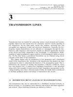
RESONANT CIRCUITS
A communication circuit designer frequently requires means to select (or reject) a
band of frequencies from a wide signal spectrum. Resonant circuits provide such
®ltering. There are well-developed,sophisticated methodologies to meet virtually
any speci®cation. However,a simple circuit suf®ces in many cases. Further,resonant
circuits are an integral part of the frequency-selective ampli®er as well as of the
oscillator designs. These networks are also used for impedance transformation and
matching.
This chapter describes the analysis and design of these simple frequency-selective
circuits,and presents the characteristic behaviors of series and parallel resonant
circuits. Related parameters,such as quality factor,bandwidth,and input impedance,
are introduced that will be used in several subsequent chapters. Transmission lines
with an open or short circuit at their ends are considered next and their relationships
with the resonant circuits are established. Transformer-coupled parallel resonant
circuits are brie¯y discussed because of their signi®cance in the radio frequency
range. The ®nal section summarizes the design procedure for rectangular and
circular cylindrical cavities,and the dielectric resonator.
4.1 SERIES RESONANT CIRCUITS
Consider the series R-L-C circuit shown in Figure 4.1. Since the inductive reactance
is directly proportional to signal frequency,it tries to block the high-frequency
contents of the signal. On the other hand,capacitive reactance is inversely propor-
tional to the frequency. Therefore,it tries to stop its lower frequencies. Note that the
voltage across an ideal inductor leads the current by 90

(i.e.,the phase angle of an
105
Radio-Frequency and Microwave Communication Circuits: Analysis and Design
Devendra K. Misra
Copyright # 2001 John Wiley & Sons,Inc.
ISBNs: 0-471-41253-8 (Hardback); 0-471-22435-9 (Electronic)

inductive reactance is 90

). In the case of a capacitor,voltage across its terminals
lags behind the current by 90

(i.e.,the phase angle of a capacitive reactance is
À90

). That means it is possible that the inductive reactance will be canceled out by
the capacitive reactance at some intermediate frequency. This frequency is called the
resonant frequency of the circuit. If the input signal frequency is equal to the
resonant frequency,maximum current will ¯ow through the resistor and it will be in
phase with the input voltage. In this case,the output voltage V
o
will be equal to the
input voltage V
in
. It can be analyzed as follows.
From Kirchhoff's voltage law,
L
R
dv
o
t
dt

1
RC

t

ÀI
v
o
tdt  v
o
tv
in
t4:1:1
Taking the Laplace transform of this equation with initial conditions as zero (i.e.,no
energy storage initially),we get
sL
R

1
sRC
 1

V
o
sV
i
s4:1:2
where s is the complex frequency (Laplace variable).
The transfer function of this circuit, Ts,is given by
Ts
V
o
s
V
i

s

1
sL
R

1
sRC
 1

sR
s
2
L  sR 
1
C
4:1:3
Therefore,the transfer function of this circuit has a zero at the origin of the complex
s-plane and also it has two poles. The location of these poles can be determined by
solving the following quadratic equation.
s
2
L  sR 
1
C
 0 4:1:4
Figure 4.1 A series R-L-C circuit with input-output terminals.
106
RESONANT CIRCUITS
Two possible solutions to this equation are as follows.

s
1;2
À
R
2L
Æ

R
2L

2
À
1
LC
s
4:1:5
The circuit response will be in¯uenced by the location of these poles. Therefore,
these networks can be characterized as follows.
 If
R
2L
>
1

LC
p
,i.e.,R > 2

L
C

r
,both of these poles will be real and distinct,and
the circuit is overdamped.
 If
R
2L

1

LC
p
,i.e.,R  2

L
C
r
,the transfer function will have double poles at
s À
R
2L
À
1

LC
p
. The circuit is critically damped.
 If
R
2L
<

1

LC
p
,i.e.,R < 2

L
C
r
,the two poles of Ts will be complex conjugate
of each other. The circuit is underdamped.
Alternatively,the transfer function may be rearranged as follows:
Ts
sCR
s
2
LC  sRC  1

sCRo
2
o
s
2
 2zo
o
s  o
2
o
4:1:6
where

z 
R
2

C
L
r
4:1:7
o
o

1

LC
p
4:1:8
z is called the damping ratio,and o
o
is the undamped natural frequency.
Poles of Ts are determined by solving the following equation.
s
2
 2zo
o
s  o
2
o
 0 4:1:9
For z < 1, s
1;2

Àzo
o
Æ jo
o

1 À z
2
p
. As shown in Figure 4.2,the two poles are
complex conjugate of each other. Output transient response will be oscillatory with a
ringing frequency of o
o
1 À z
2
 and an exponentially decaying amplitude. This
circuit is underdamped.
For z  0,the two poles move on the imaginary axis. Transient response will be
oscillatory. It is a critically damped case.
For z  1,the poles are on the negative real axis. Transient response decays
exponentially. In this case,the circuit is overdamped.
SERIES RESONANT CIRCUITS
107
Consider the unit step function shown in Figure 4.3. It is like a direct voltage
source of one volt that is turned on at time t  0. If it represents input voltage v
in
t
then the corresponding output v
o
t can be determined via Laplace transform
technique.

The Laplace transform of a unit step at the origin is equal to 1=s. Hence,output
voltage, v
o
t,is found as follows.
v
o
tL
À1
V
o
sL
À1
sCRo
2
o
s
2
 2zo
o
s  o
2
o
Â
1
s
 L
À1
CRo
2
o

s  zo
o

2
1À z
2
o
2
o
where L
À1
represents inverse Laplace transform operator. Therefore,
v
o
t
2B

1 À z
2
p
e
ÀBo
o
t
sin o
o
t

1 À z
2

q

ut
Figure 4.2 Pole-zero plot of the transfer function.
Figure 4.3 A unit-step input voltage.
108
RESONANT CIRCUITS
This response is illustrated in Figure 4.4 for three different damping factors. As
can be seen,initial ringing lasts longer for a lower damping factor.
A sinusoidal steady-state response of the circuit can be easily determined after
replacing s by jo,as follows:
V
o
 jo
V
i
 jo
joL
R

1
joRC
 1

V
i
 jo
1 
j
RC

LCo À
1
o

or,
V
o
 jo
V
i
 jo
1 
j
RC
o
o
2
o
À
1
o


V
i
 jo
1 
j
o
o

RC
o
o
o
À
o
o
o

The quality factor, Q,of the resonant circuit is a measure of its frequency selectivity.
It is de®ned as follows.
Q  o
o
Average stored energy
Power loss
4:1:10
Figure 4.4 Response of a series R-L-C circuit to a unit step input for three different damping
factors.
SERIES RESONANT CIRCUITS
109
Hence,
Q  o
o
1
2
LI
2
1
2
I

2
R

o
o
L
R
Since o
o
L 
1
o
o
C
,
Q 
o
o
L
R

1
o
o
RC


LC
p
RC


1
R

L
C
r

1
2z
4:1:11
Therefore,
V
o
 jo
V
i
 jo
1  jQ
o
o
o
À
o
o
o

4:1:12
Alternatively,
V

o
 jo
V
i
 jo
 A jo
1
1  jQ
o
o
o
À
o
o
o

4:1:13
The magnitude and phase angle of (4.1.13) are illustrated in Figures 4.5 and 4.6,
respectively. Figure 4.5 shows that the output voltage is equal to the input for a
signal frequency equal to the resonant frequency of the circuit. Further,phase angles
of the two signals in Figure 4.6 are the same at this frequency,irrespective of the
quality factor of the circuit. As signal frequency moves away from this point on
either side,the output voltage decreases. The rate of decrease depends on the quality
factor of the circuit. For higher Q,the magnitude is sharper,indicating a higher
selectivity of the circuit. If signal frequency is below the resonant frequency then
output voltage leads the input. For a signal frequency far below the resonance,output
leads the input almost by 90

. On the other hand,it lags behind the input for higher
frequencies. It converges to À90


as the signal frequency moves far beyond the
resonant frequency. Thus,the phase angle changes between p=2 and Àp=2,
following a sharper change around the resonance for high-Q circuits. Note that
the voltage across the series-connected inductor and capacitor combined has inverse
characteristics to those of the voltage across the resistor. Mathematically,
V
LC
 joV
in
 joÀV
o
 jo
110
RESONANT CIRCUITS
Figure 4.5 Magnitude of A jo as a function of o.
Figure 4.6 The phase angle of A jo as a function of o.
SERIES RESONANT CIRCUITS
111
where V
LC
 jo is the voltage across the inductor and capacitor combined. In this
case,sinusoidal steady-state response can be obtained as follows.
V
LC
 jo
V
in
 jo
 1 À

V
o
 jo
V
in
 jo
 1 À
1
1  jQ
o
o
o
À
o
o
o


jQ
o
o
o
À
o
o
o

1  jQ
o
o

o
À
o
o
o

Hence,this con®guration of the circuit represents a band-rejection ®lter.
Half-power frequencies o
1
and o
2
of a band-pass circuit can be determined from
(4.1.13) as follows:
1
2

1
1  Q
2
o
o
o
À
o
o
o

2
A 2  1  Q
2

o
o
o
À
o
o
o

2
Therefore,
Q
o
o
o
À
o
o
o

Æ1
Assuming that o
1
< o
o
< o
2
,
Q
o
1

o
o
À
o
o
o
1

À1
and,
Q
o
2
o
o
À
o
o
o
2

 1
Therefore,
o
2
o
o
À
o
o

o
2
À
o
1
o
o
À
o
o
o
1

or,
o
2
À
o
2
o
o
2
Ào
1

o
2
o
o
1

Ao
2
 o
1

o
2
o
o
1

o
2
o
o
1
 o
2
o
1
o
1

1
o
2

or,
o
2

o
 o
1
o
2
4:1:14
112
RESONANT CIRCUITS
and,
o
1
o
o
À
o
o
o
1

À
1
Q
A o
1
À
o
2
o
o
1

À
o
o
Q
or,
o
1
À o
2
À
o
o
Q
A Q 
o
o
o
2
À o
1
4:1:15
Example 4.1: Determine the element values of a resonant circuit that passes all the
sinusoidal signals from 9 MHz to 11 MHz. This circuit is to be connected between a
voltage source with negligible internal impedance and a communication system with
its input impedance at 50 O. Plot its characteristics in a frequency band of 1 to
20 MHz.
From (4.1.14),
o
o



o
1
 o
2
p
3 f
o


f
1
 f
2
p


9 Â 11
p
 9:949874 MHz
From (4.1.11) and (4.1.15),
Q 
o
o
L
R

o
o
o

1
À o
2
3 L 
R
o
1
À o
2

50
2  p  10
6
Â11À 9
 3:978874 Â 10
À6
H % 4 mH
From (4.1.8),
o
o

1

LC
p
A C 
1
Lo
2
o

 6:430503 Â 10
À11
F % 64:3pF
The circuit arrangement is shown in Figure 4.7. Its magnitude and phase
characteristics are displayed in Figure 4.8.
Figure 4.7. The ®lter circuit arrangement for Example 4.1.
SERIES RESONANT CIRCUITS
113
Input Impedance
Impedance across the input terminals of a series R-L-C circuit can be determined as
follows.
Z
in
 R  joL 
1
joC
 R  joL 1 À
o
2
o
o
2

4:1:16
Figure 4.8 Magnitude (a) and phase (b) plots of A ( jo) for the circuit in Figure 4.7.
114
RESONANT CIRCUITS
At resonance,the inductive reactance cancels out the capacitive reactance.
Therefore,the input impedance reduces to total resistance of the circuit. If signal
frequency changes from the resonant frequency by Ædo,the input impedance can be

approximated as follows.
Z
in
 R  joL
o  o
o
o À o
o

o
2
% R  j2doL  R  j
2QRdo
o
o
4:1:17
Alternatively,
Z
in
% R  j2doL 
o
o
L
Q
 j2o À o
o
L  j2 o À o
o

o

o
j2Q

L
 j2 o À o
o
1  j
1
2Q

L 4:1:18
Therefore,a series resonant circuit can be analyzed with R as zero (i.e.,assuming
that the circuit is lossless). The losses can be included subsequently by replacing a
real resonant frequency, o
o
,by the complex frequency,o
o
1  j
1
2Q

.
At resonance,current through the circuit,I
r
,
I
r

V
in

R
4:1:19
Therefore,voltages across the inductor,V
L
,and the capacitor,V
c
,are
V
L
 jo
o
L
V
in
R
 jQV
in
4:1:20
and,
V
C

1
jo
o
C
V
in
R
ÀjQV

in
4:1:21
Hence,the magnitude of voltage across the inductor is equal to the quality factor
times input voltage while its phase leads 90

. Magnitude of the voltage across the
capacitor is the same as that across the inductor. However,it is 180

out of phase
because it lags behind the input voltage by 90

.
4.2 PARALLEL RESONANT CIRCUITS
Consider an R-L-C circuit in which the three components are connected in parallel,
as shown in Figure 4.9. A subscript p is used to differentiate the circuit elements
from those used in the series circuit of the preceding section. A current source, i
in
t,
PARALLEL RESONANT CIRCUITS
115
is connected across its terminals and i
o
t is current through the resistor R
p
. Voltage
across this circuit is v
o
t. From Kirchhoff's current law,
i
in

t
1
L
p

t
ÀI
R
p
i
o
tdt  C
p
dR
p
i
o
t
dt
 i
o
t4:2:1
Assuming that there was no energy stored in the circuit initially,we take the
Laplace transform of (4.2.1). It gives
I
in
s
R
p
sL

p
 sR
p
C
p
 1
!
I
o
s
Hence,
I
o
s
I
in
s

sL
p
R
p
s
2
L
p
C
p
 s
L

p
R
p
 1
!
4:2:2
Note that this equation is similar to (4.1.6) of the preceding section. It changes to
Ts if RC replaces L
p
=R
p
. Therefore,results of the series resonant circuit can be
used for this parallel resonant circuit,provided
z 
1
2o
o
R
p
C
p
and,
o
o

1

L
p
C

p
p
4:2:3
Hence,
z 
1
2o
o
R
p
C
p

1
2R
p

L
p
C
p
s
4:2:4
Figure 4.9 A parallel R-L-C circuit.
116
RESONANT CIRCUITS
The quality factor, Q
p
,and the impedance,Z
p

,of the parallel resonant circuit can
be determined as follows:
Q
series

o
o
L
R

1
o
o
RC
A Q
p
 o
o
R
p
C
p

R
p
o
o
L
p
4:2:5

Z
p

V
o
 jo
I
in
io

I
o
 joR
p
I
in
 jo

joL
p
Ào
2
L
p
C
p
 jo
L
p
R

p
 1
!
4:2:6
Input Admittance
Admittance across input terminals of the parallel resonant circuit (i.e.,the admittance
seen by the current source) can be determined as follows.
Y
in

1
Z
p

1
R
p
 joC
p

1
joL
p

1
R
p
 joC
p
1 À

o
2
o
o
2

4:2:7
Hence,input admittance will be equal to 1=R
p
at the resonance. It will become zero
(that means the impedance will be in®nite) for a lossless circuit. It can be
approximated around the resonance, o
o
Æ do,as follows.
Y
in
%
1
R
p
 j2doC
p

1
R
p
 j
2doQ
o
o

R
p
4:2:8
The corresponding impedance is
Z
p
%
R
p
1  j
2Qdo
o
o
4:2:9
Current through the capacitor, I
c
,at the resonance is
I
c
 jo
o
C
p
R
p
I
in
 jQI
in
4:2:10

and current through the inductor, I
L
,is
I
L

1
jo
o
L
p
R
p
I
in
ÀjQI
in
4:2:11
Thus,current through the inductor is equal in magnitude but opposite in phase to
that through the capacitor. Further,these currents are larger than the input current by
a factor of Q.
Quality Factor of a Resonant Circuit
If resistance R represents losses in the resonant circuit, Q given by the preceding
formulas is known as the unloaded Q. If the power loss due to external load coupling
PARALLEL RESONANT CIRCUITS
117
is included through an additional resistance R
L
then the external Q
e

is de®ned as
follows:
Q
e

o
o
L
R
L
for series resonant circuit
R
L
o
o
L
p
for parallel resonant circuit
8
>
>
>
<
>
>
>
:
4:2:12
The loaded Q, Q
L

,of a resonant circuit includes internal losses as well as the
power extracted by the external load. It is de®ned as follows:
Q
L

o
o
L
R
L
 R
for series resonant circuit
R
L
kR
p
o
o
L
p
for parallel resonant circuit
8
>
>
>
<
>
>
>
:

4:2:13
where,
R
L
kR
p

R
L
R
p
R
L
 R
p
Hence,the following relation holds good for both kinds of resonant circuits (see
Table 4.1).
1
Q
L

1
Q
e

1
Q
4:2:14
Example 4.2: Consider the loaded parallel resonant circuit illustrated here.
Compute the resonant frequency in radians per second,unloaded Q,and the

loaded Q of this circuit.
o
o

1

L
p
C
p
p

1

10
À5
 10
À11
p
 10
8
rad=s
The unloaded Q 
R
p
o
o
L
p


10
5
10
8
 10
À5
 100.
118
RESONANT CIRCUITS
The external Q; Q
e

R
L
o
o
L
p

10
5
10
8
 10
À5
 100.
The loaded Q; Q
L

R

p
kR
L
o
o
L
p

QQ
e
Q  Q
e

50 Â 10
3
10
8
 10
À5
 50 .
4.3 TRANSFORMER-COUPLED CIRCUITS
Transformers are used as a means of coupling as well as of impedance transforming
in electronic circuits. Transformers with tuned circuits in one or both of their sides
are employed in voltage ampli®ers and oscillators operating at radio frequencies.
This section presents an equivalent model and an analytical procedure for the
transformer-coupled circuits.
Consider a load impedance Z
L
that is coupled to the voltage source V
s

via a
transformer as illustrated in Figure 4.10. Source impedance is assumed to be Z
s
. The
transformer has a turn ratio of n:1 between its primary (the source) and secondary
(the load) sides.
Using the notations as indicated,equations for various voltages and currents can
be written in phasor form as follows.
V
1
 joL
1
I
1
 joMI
2
4:3:1
V
2
 joMI
1
 joL
2
I
2
4:3:2
TABLE 4.1 Relations for Series and Parallel Resonant Circuits
Series Parallel
o
o

1

LC
p
1

L
p
C
p
p
Damping factor, z
R
2

C
L
r
1
2R
p

L
p
C
p
s
Unloaded Q
o
o

L
R

1
o
o
RC
R
p
o
o
L
p
 o
o
R
p
C
p
External Q  Q
e
o
o
L
R
L

1
o
o

R
L
C
R
L
o
o
L
p
 o
o
R
L
C
p
Loaded Q  Q
L
Q Â Q
e
Q  Q
e
Q Â Q
e
Q  Q
e
Input impedance, Z
in
,around resonance R  j
2RQdo
o

o
R
1  j
2Qdo
o
o
TRANSFORMER-COUPLED CIRCUITS
119
where M is the mutual inductance between the two sides of the transformer.
Standard convention with a dot on each side is used. Hence,magnetic ¯uxes
reinforce each other for the case of currents entering this terminal on both sides,and
M is positive.
The following relations hold for an ideal transformer operating at any frequency.
V
1
 nV
2
4:3:3
I
1
À
I
2
n
4:3:4
and,
V
1
I
1

 Z
1

nV
2
ÀI
2
=n
 n
2
V
2
ÀI
2
 n
2
Z
2
4:3:5
There are several equivalent circuits available for a transformer. We consider one
of these that is most useful in analyzing the communication circuits. This equivalent
circuit is illustrated in Figure 4.11 below. The following equations for phasor
voltages and currents may be formulated using the notations indicated in Figure
4.11.
V
1
 jo1 À xL
1
I
1

 joxL
1
I
1

I
2
n

 joL
1
I
1
 joxL
1
I
2
n
4:3:6
and,
V
2

1
n
joxL
1
I
1


I
2
n

4:3:7
If the circuit shown in Figure 4.11 is equivalent to that shown in Figure 4.10 then
these two equations represent the same voltages as those of (4.3.1) and (4.3.2).
Figure 4.10 A transformer-coupled circuit.
120
RESONANT CIRCUITS