Tài liệu Data Preparation for Data Mining- P10 docx

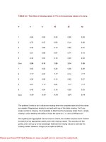
TABLE 8.3 The effect of missing values (?.??) on the summary values of x and y.







n




x





y





x2

y2





xy








1




0.55





0.53

0.30





0.28





0.29





2




0.75

0.37





0.56





0.14





0.28





3

0.32





0.83





0.10





0.69





0.27

4




0.21





0.86





0.04





0.74

0.18





5




0.43





0.54





0.18

0.29





0.23





Sum




2.26





3.13





1.20

2.14





1.25





1




0.55





0.53

0.30





0.28





0.29





2




?.??

0.37





?.??





0.14





?.??





3

0.32





0.83





0.10





0.69





0.27

4




0.21





?.??





0.04





?.??

?.??





5




0.43





0.54





0.18

0.29





0.23





Sum




?.??





?.??





?.??

?.??





?.??








The problem is what to do if values are missing when the complete totals for all the values
are needed. Regressions simply do not work with any of the totals missing. Yet if any
single number is missing, it is impossible to determine the necessary totals. Even a single
missing x value destroys the ability to know the sums for x, x
2
, and xy! What to do?

Since getting the aggregated values correct is critical, the modeler requires some method
to determine the appropriate values, even with missing values. This sounds a bit like
pulling one’s self up by one’s bootstraps! Estimate the missing values to estimate the
missing values! However, things are not quite so difficult.


Please purchase PDF Split-Merge on www.verypdf.com to remove this watermark.


In a representative sample, for any particular joint distribution, the ratios between the
various values xx and xx
2
, and xy and xy
2
remain constant. So too do the ratios between
xx and xxy and xy and xxy. When these ratios are found, they are the equivalent of setting
the value of n to 1. One way to see why this is so is because in any representative sample
the ratios are constant, regardless of the number of instance values—and that includes
n = 1. More mathematically, the effect of the number of instances cancels out. The end
result is that when using ratios, n can be set to unity. In the linear regression formulae,
values are multiplied by n, and multiplying a value by 1 leaves the original value
unchanged. When multiplying by n = 1, the n can be left out of the expression. In the
calculations that follow, that piece is dropped since it has no effect on the result.




The key to building the regression equations lies in discovering the needed ratios for
those values that are jointly present. Given the present and missing values that are shown
in the lower part of Table 8.3, what are the ratios?

Table 8.4 shows the ratios determined from the three instance values where x and y are
both present. Using the expressions for linear regression and these ratios, what is the
estimated value for the missing y value from Table 8.3?




TABLE 8.4 Ratios of the values that are present in the lower part of Table 8.3.










xx2





xy2

xxy








Ratio xx to:




0.45









0.61

Ratio xy to:








0.66





0.42








In addition to the ratios, the sums of the x and y values that are present need to be found.
But since the ratios scale to using an n of 1, so too must the sums of x and y—which is

identical to using their mean values. The mean values of variable x and of variable y are
taken for the values of each that are jointly present as shown in Table 8.5.




TABLE 8.5 Mean values of x and y for estimating missing values.







n




x





y



Please purchase PDF Split-Merge on www.verypdf.com to remove this watermark.

1




0.55





0.53





2

0.37





3




0.32





0.83





4




0.21

5




0.43





0.54





Sum

1.30





1.90





Mean




0.43





0.63

For the linear regression, first a value for b must be found. Because ratios are being used,
the ratio must be used to yield an appropriate value of xx
2
and xxy to use for any value of
xx. For example, since the ratio of xx to xx
2
is 0.45, then given an xx of 0.43, the
appropriate value of xx
2
is 0.43 x 0.45 = 0.1935—that is, the actual value multiplied by the
ratio. Table 8.6 shows the appropriate values to be used with this example of a missing x
value.




TABLE 8.6 Showing ratio-derived estimated values for xx2 and xxy.







Est xx

Est xx
2






Est xxy








0.43




0.43 x 0.45 = 0.1935

0.43 x 0.61 = 0.2623








Plugging these values into the expression to find b gives



Please purchase PDF Split-Merge on www.verypdf.com to remove this watermark.






So b = –1. The negative sign indicates that values of y will decrease as values of x
increase. Given this value for b, a can be found:

The a value is 1.06. With suitable values discovered for a and b, and using the formula for
a straight line, an expression can be built that will provide an appropriate estimate for any
missing value of y, given a value of x. That expression is




y = a + bx




y = 1.06 + (–1)x




y = 1.06 – x




Table 8.7 uses this expression to estimate the values of y, given x, for all of the original
values of x.




TABLE 8.7 Derived estimates of y given an x value using linear regression based

on ratios.







Original x




Original y





Estimated y





Error

0.55




0.53





0.51





0.02





0.75

0.37





0.31





0.06



Please purchase PDF Split-Merge on www.verypdf.com to remove this watermark.


0.32




0.83

0.74





0.09





0.21




0.86





0.85

0.01





0.43




0.54





0.63





0.09

These estimates of y are quite close to the original values in this example. The error, the
difference between the original value and the estimate, is small compared to the actual
value.




Multiple Linear Regression




The equations used for performing multiple regression are extensions of those already
used for linear regression. They are built from the same components as linear
regression—xx, xx
2
, xxy—for every pair of variables included in the multiple regression.
(Each variable becomes x in turn, and for that x, each of the other variables becomes y in
turn.) All of these values can be estimated by finding the ratio relationships for those
variables’ values that are jointly present in the initial sample data set. With this information
available, good linear estimates of the missing values of any variable can be made using
whatever variable instance values are actually present.




With the ratio information known for all of the variables, a suitable multiple regression can

be constructed for any pattern of missing values, whether it was ever experienced before
or not. Appropriate equations for the instance values that are present in any instance can
be easily constructed from the ratio information. These equations are then used to predict
the missing values.




For a statistician trying to build predictions, or glean inferences from a data set, this
technique presents certain problems. However, the problems facing the modeler when
replacing data are very different, for the modeler requires a computationally tractable
method that introduces as little bias as is feasible when replacing missing values. The
missing-value replacements themselves should contribute no information to the model.
What they do is allow the information that is present (the nonempty instance values) to be
used by the modeling tool, adding as little extraneous distortion to a data set as possible.




It may seem strange that the replacement values should contribute no information to a
data set. However, any replacement value can only be generated from information that is
already present in the form of other instance values. The regression equations fit the
replacement value in such a way that it least distorts the linear relationships already
discovered. Since the replacement value is derived exclusively from information that is
already present in the data set, it can only reexpress the information that is already

Please purchase PDF Split-Merge on www.verypdf.com to remove this watermark.
present. New information, being new, changes what is already known to a greater or
lesser degree, actually defining the relationship. Replacement values should contribute as
little as possible to changing the shape of the relationships that already exist. The existing

relationship is what the modeler needs to explore, not some pattern artificially constructed
by replacing missing values!



Alternative Methods of Missing-Value Replacement




Preserving joint variability between variables is far more effective at providing unbiased
replacement values than methods that do not preserve variability. In practice, many
variables do have essentially linear between-variable relationships. Even where the
relationship is nonlinear, a linear estimate, for the purpose of finding a replacement for a
missing value, is often perfectly adequate. The minute amount of bias introduced is often
below the noise level in the data set anyway and is effectively unnoticeable.




Compared to finding nonlinear relationships, discovering linear relationships is both fast
and easy. This means that linear techniques can be implemented to run fast on modern
computers, even when the dimensionality of a data set is high. Considering the small
amount of distortion usually associated with linear techniques, the trade-offs in terms of
speed and flexibility are heavily weighted in favor of their use. The replacement values
can be generated dynamically (on the fly) at run time and substituted as needed.

However, there are occasions when the relationship is clearly nonlinear, and when a
linear estimate for a replacement value may introduce significant bias. If the modeler
knows that the relationship exists, some special replacement procedure for missing
values can be used. The real problem arises when a significantly nonlinear relationship
exists that is unknown to the modeler and domain expert. Mining will discover this
relationship, but if there are missing values, linear estimates for replacements will produce
bias and distortion. Addressing these problems is outside the scope of the demonstration
software, which is intended only to illustrate the principles involved in data preparation.




There are several possible ways to address the problem. Speed in finding replacement
values is important for deployed production systems. In a typical small direct marketing
application, for instance, a solicitation mailing model may require replacing anything from
1 million to 20 million values. As another example, large-scale, real-time fraud detection
systems may need from tens to hundreds of millions of replacement values daily.




Tests of Nonlinearity: Extending the Ratio Method of Estimation




There are tests to determine nonlinearity in a relationship. One of the easiest is to simply
try nonlinear regressions and see if the fit is improved as the nonlinearity of the
expression increases. This is certainly not foolproof. Highly nonlinear relationships may
well not gradually improve their fit as the nonlinearity of the expression is increased.

Please purchase PDF Split-Merge on www.verypdf.com to remove this watermark.

An advantage of this method is that the ratio method already described can be extended
to capture nonlinear relationships. The level of computational complexity increases
considerably, but not as much as with some other methods. The difficulty is that choosing
the degree of nonlinearity to use is fairly arbitrary. There are robust methods to determine
the amount of nonlinearity that can be captured at any chosen degree of nonlinearity
without requiring that the full nonlinear multiple regressions be built at every level. This
allows a form of optimization to be included in the nonlinearity estimation and capture.
However, there is still no guarantee that nonlinearities that are actually present will be
captured. The amount of data that has to be captured is quite considerable but relatively
modest compared with other methods, and remains quite tractable.




At run time, missing-value estimates can be produced very quickly using various
optimization techniques. The missing-value replacement rate is highly dependent on
many factors, including the dimensionality of the data set and the speed of the computer,
to name only two. However, in practical deployed production systems, replacement rates
exceeding 1000 replacements per second, even in large or high-throughput data sets,
can be easily achieved on modern PCs.




Nonlinear Submodels

Another method of capturing the nonlinearities is to use a modeling tool that supports
such a model. Neural networks work well (described briefly in Chapter 10). In this case,
for each variable in the data set, a subsample is created that has no missing values. This
is required as unmodified neural networks do not handle missing values—they assume
that all inputs have some value. A predictive model for every variable is constructed from
all of the other variables, and for the MVPs. When a missing value is encountered, the
appropriate model is used to predict its value from the available variable values.




There are significant drawbacks to such a method. The main flaw is that it is impossible to
train a network for every possible pattern of missing values. Training networks for all of
the detected missing patterns in the sample may itself be an enormous task. Even when
done, there is no prediction possible when the population produces a previously
unencountered MVP, since there is no network trained for that configuration. Similarly, the
storage requirements for the number of networks may be unrealizable.




A modification of this method builds fewer models by using subsets of variables as inputs.
If the subset inputs are carefully selected, models can be constructed that among them
have a very high probability that at least one of them will be applicable. This approach
requires constructing multiple, relatively small networks for each variable. However, such
an approach can become intractable very quickly as dimensionality of the data set

increases.




An additional problem is that it is hard to determine the appropriate level of complexity.
Missing-value estimates are produced slowly at run time since, for every value, the

Please purchase PDF Split-Merge on www.verypdf.com to remove this watermark.
appropriate network has to be looked up, loaded, run, and output produced.



Autoassociative Neural Networks




Autoassociative neural networks are briefly described in Chapter 10. In this architecture,
all of the inputs are also used as predicted outputs. Using such an architecture, only a
single neural network need be built. When a missing value(s) is detected, the network can
be used in a back-propagation mode—but not a training mode, as no internal weights are
adjusted. Instead, the errors are propagated all the way back to the inputs. At the input, an
appropriate weight can be derived for the missing value(s) so that it least disturbs the
internal structure of the network. The value(s) so derived for any set of inputs reflects, and
least disturbs, the nonlinear relationship captured by the autoassociative neural network.

As with any neural network, its internal complexity determines the network’s ability to
capture nonlinear relationships. Determining that any particular network has, in fact,
captured the extant nonlinear relationship is difficult. The autoassociative neural network
approach has been used with success in replacing missing values for data sets of modest
dimensionality (tens and very low hundreds of inputs), but building such networks for
moderate- to high-dimensionality data sets is problematic and slow. The amount of data
required to build a robust network becomes prohibitive, and for replacement value
generation a robust network that actually reflects nonlinearities is needed.




At run time, replacement values can be produced fairly quickly.




Nearest-Neighbor Estimators




Nearest-neighbor methods rely on having the training set available at run time. The
method requires finding the point in state space best represented by the partially
complete instance value, finding the neighbors nearest to that point, and using some
metric to derive the missing values. It depends on the assumption that representative
near neighbors can be found despite the fact that one or more dimensional values is
missing. This can make it difficult to determine a point in state space that is
representative, given that its position in the dimensions whose value is missing is
unknown. Nonetheless, such methods can produce good estimates for missing values.

Such methods are inherently nonlinear so long as representative near neighbors can be
found.




The main drawbacks are that having the training data set available, even in some collapsed
form, may require very significant storage. Lookup times for neighbors can be very slow, so
finding replacement values too is slow.


Please purchase PDF Split-Merge on www.verypdf.com to remove this watermark.

Chapter 9: Series Variables




Overview




Series variables have a number of characteristics that are sufficiently different from other
types of variables that they need examining in more detail. Series variables are always at
least two-dimensional, although one of the dimensions may be implicit. The most common
type of series variable is a time series, in which a series of values of some feature or
event are recorded over a period of time. The series may consist of only a list of
measurements, giving the appearance of a single dimension, but the ordering is by time,
which, for a time series, is the implicit variable.

The series values are always measured on one of the scales already discussed, nominal
through ratio, and are presented as an ordered list. It is the ordering, the expression of the
implied variable, that requires series data to be prepared for mining using techniques in
addition to those discussed for nonseries data. Without these additional techniques the
miner will not be able to best expose the available information. This is because series
variables carry additional information within the ordering that is not exposed by the
techniques discussed so far.




Up to this point in the book we have developed precise descriptions of features of
nonseries data and various methods for manipulating the identified features to expose
information content. This chapter does the same for series data and so has two main
tasks:




1.

Find unambiguous ways to describe the component features of a series data set so
that it can be accurately and completely characterized

2.

Find methods for manipulating the unique features of series data to expose the
information content to mining tools




Series data has features that require more involvement by the miner in the preparation
process than for nonseries data. Where miner involvement is required, fully automated
preparation tools cannot be used. The miner just has to be involved in the preparation and
exercise judgment and experience. Much of the preparation requires visualizing the data set
and manipulating the series features discussed. There are a number of excellent commercial
tools for series data visualization and manipulation, so the demonstration software does not
include support for these functions. Thus, instead of implementation notes concluding the
chapter discussing how the features discussed in the chapter are put into practice, this
chapter concludes with a suggested checklist of actions for preparing series data for the
miner to use.


Please purchase PDF Split-Merge on www.verypdf.com to remove this watermark.
9.1 Here There Be Dragons!




Mariners and explorers of old used fanciful and not always adequate maps. In unexplored or
unknown territory, the map warned of dragons—terrors of the unknown. So it is when
preparing data, for the miner knows at least some of the territory. Many data explorers have

passed this way. A road exists. Signposts point the way. Maybe the dragons were chased
away, but still be warned. “Danger, quicksand!” Trouble lurks inside series data; the road of
data preparation is rocky and uncertain, sometimes ending mired in difficulties. It is all too
easy to seriously damage data, render it useless, or worse, create wonderful-looking
distortions that are but chimera that melt away when exposed to the bright light of reality.
Like all explorers faced with uncertainty, the miner needs to exercise care and experience
here more than elsewhere. The road is rough and not always well marked. Unfortunately, the
existing signposts, with the best of intentions, can still lead the miner seriously astray. Tread
this path with caution!


9.2 Types of Series




Nonseries multivariable measurements are taken without any particular note of their
ordering. Ordering is a critical feature of a series. Unless ordered, it’s not a series. One of
the variables (called the displacement variable, and described in a moment) is always
monotonic—either constantly increasing or constantly decreasing. Whether there is one
or several other variables in the series, their measurements are taken at defined points on
the range of the monotonic variable. The key ordering feature is the change in the
monotonic variable as its values change across part or all of its range.




Time series are by far the most common type of series. Measurements of one variable are
taken at different times and ordered such that an earlier measurement always comes
before a later measurement. For a time series, time is the displacement variable—the

measurements of the other variable (or variables) are made as time is “displaced,” or
changed. The displacement variable is also called the index variable. That is because the
points along the displacement variable at which the measurements are taken are called
the index points.




Dimensions other than time can serve as the displacement dimension. Distance, for
instance, can be used. For example, measuring the height of the American continent
above sea level at different points on a line extending from the Atlantic to the Pacific
produces a distance displacement series.




Since time series are the most common series, where this chapter makes assumptions, a
time series will be assumed. The issues and techniques described about time series also
apply to any other displacement series. Series, however indexed, share many features in
common, and techniques that apply to one type of series usually apply to other types of
series. Although the exact nature of the displacement variable may make little difference to
the preparation and even, to some degree, the analysis of the series itself, it makes all the
Please purchase PDF Split-Merge on www.verypdf.com to remove this watermark.
difference to the interpretation of the result!


9.3 Describing Series Data

Series data differs from the forms of data so far discussed mainly in the way in which the
data enfolds the information. The main difference is that the ordering of the data carries
information. This ordering, naturally, precludes random sampling since random sampling
deliberately avoids, and actually destroys, any ordering. Preserving the ordering is the
main reason that series data has to be prepared differently from nonseries data.




There is a large difference between preparing data for modeling and actually modeling the
data. This book focuses almost entirely on how to prepare the data for modeling, leaving
aside almost all of the issues about the actual modeling, insofar as is practical. The same
approach will apply to series data. Some of the tools needed to address the data
preparation problems may look similar, indeed are similar, to those used to model and
glean information and insight into series data. However, they are put to different purposes
when preparing data. That said, in order to understand some of the potential problems
and how to address them, some precise method of describing a series is needed. A key
question is, What are the features of series data?




To answer this question, the chapter will first identify some consistent, recognizable, and
useful features of series data. The features described have to be consistent and
recognizable as well as useful. The useful features are those that best help the miner in
preparing series data for modeling. The miner also needs these same features when
modeling. This is not surprising, as finding the best way to expose the features of interest
for modeling is the main objective of data preparation.

9.3.1 Constructing a Series




A series is constructed by measuring and recording a feature of an object or event at
defined index points on a displacement dimension.




This statement sufficiently identifies a series for mining purposes. It is not a formal
definition but a conceptual description, which also includes the following assumptions:




1.

The feature or event is recorded as numerical information.




2.

The index point information is either recorded, or at least the displacements are

defined.




3.

The index, if recorded, is recorded numerically.




It is quite possible to record a time series using alpha labels for the nondisplacement
dimension, but this is extremely rare. Numerating such alpha values within the series is

Please purchase PDF Split-Merge on www.verypdf.com to remove this watermark.
possible, although it requires extremely complex methods. While it is very unusual indeed
to encounter series with one alpha dimension, it is practically unknown to find a series
with an alpha-denominated displacement variable. The displacement dimension has to be
at least an ordinal variable (ratio more likely), and these are invariably numerical.
Because series with all dimensions numerical are so prevalent, we will focus entirely on
those.



It is also quite possible to record multivariable series sharing a common displacement
variable, in other words, capturing several features or events at each index mark. An
example is collecting figures for sales, backlog, new orders, and inventory level every
week. “Time” is the displacement variable for all the measurements, and the index point is
weekly. The index point corresponds to the validating event referred to in Chapter 2.

There is no reason at all why several features should not be captured at each index, the
same as in any nonseries multidimensional data set. However, just as each of the
variables can be considered separately from each other during much of the nonseries
data preparation process, so too can each series variable in a multidimensional series be
considered separately during preparation.




9.3.2 Features of a Series




By its nature a series has some implicit pattern within the ordering. That pattern may
repeat itself over a period. Often, time series are thought of by default as repetitive, or
cyclic, but there is no reason that any repeating pattern should in fact exist. There is, for
example, a continuing debate about whether the stock market exhibits a repetitive pattern
or is simply the result of a random walk (touched on later). Enormous effort has been put
into detecting any cyclic pattern that may exist, and still the debate continues. There is,
nonetheless, a pattern in series data, albeit not necessarily a repeating one. One of the
objectives of analyzing series data is to describe that pattern, identify it as recognizable if
possible, and find any parts that are repetitive. Preparing series data for modeling, then,
must preserve the nature of the pattern that exists. Preparation also includes putting the
data into a form in which the desired information is best exposed to a modeling tool. Once
again, a warning: this is not always easy!

Before looking at how series data may be prepared, and what problems may be detected
and corrected, the focus now turns to finding some way to unambiguously describe the
series.




9.3.3 Describing a Series—Fourier




Jean Baptiste Joseph Fourier was not a professional mathematician. Nonetheless, he
exerted an influence on mathematicians and scientists of his day second only to that of Sir
Isaac Newton. Until Fourier revealed new tools for analyzing data, several scientists
lamented that the power of mathematics seemed to be just about exhausted. His insights
reinvigorated the field. Such is the power of Fourier’s insight that its impact continues to

Please purchase PDF Split-Merge on www.verypdf.com to remove this watermark.