Tài liệu Handbook of Mechanical Engineering Calculations P7 docx

P
•
A
•
R
•
T2
PLANT AND
FACILITIES
ENGINEERING
Downloaded from Digital Engineering Library @ McGraw-Hill (www.digitalengineeringlibrary.com)
Copyright © 2006 The McGraw-Hill Companies. All rights reserved.
Any use is subject to the Terms of Use as given at the website.
Source: HANDBOOK OF MECHANICAL ENGINEERING CALCULATIONS
Downloaded from Digital Engineering Library @ McGraw-Hill (www.digitalengineeringlibrary.com)
Copyright © 2006 The McGraw-Hill Companies. All rights reserved.
Any use is subject to the Terms of Use as given at the website.
PLANT AND FACILITIES ENGINEERING
7.3
SECTION 7
PUMPS AND
PUMPING SYSTEMS
PUMP OPERATING MODES AND
CRITICALITY
7.3
Series Pump Installation Analysis
7.3
Parallel Pumping Economics
7.5
Using Centrifugal Pump Specific
Speed to Select Driver Speed

7.10
Ranking Equipment Criticality to
Comply with Safety and
Environmental Regulations
7.12
PUMP AFFINITY LAWS, OPERATING
SPEED, AND HEAD
7.16
Similarity or Affinity Laws for
Centrifugal Pumps
7.16
Similarity or Affinity Laws in
Centrifugal Pump Selection
7.17
Specific Speed Considerations in
Centrifugal Pump Selection
7.18
Selecting the Best Operating Speed
for a Centrifugal Pump
7.19
Total Head on a Pump Handling
Vapor-Free Liquid
7.21
Pump Selection for any Pumping
System
7.26
Analysis of Pump and System
Characteristic Curves
7.33
Net Positive Suction Head for Hot-

Liquid Pumps
7.41
Condensate Pump Selection for a
Steam Power Plant
7.43
Minimum Safe Flow for a Centrifugal
Pump
7.46
Selecting a Centrifugal Pump to
Handle a Viscous Liquid
7.47
Pump Shaft Deflection and Critical
Speed
7.49
Effect of Liquid Viscosity on
Regenerative-Pump Performance
7.51
Effect of Liquid Viscosity on
Reciprocating-Pump Performance
7.52
Effect of Viscosity and Dissolved Gas
on Rotary Pumps
7.53
Selection of Materials for Pump Parts
7.56
Sizing a Hydropneumatic Storage
Tank
7.56
Using Centrifugal Pumps as Hydraulic
Turbines

7.57
Sizing Centrifugal-Pump Impellers for
Safety Service
7.62
Pump Choice to Reduce Energy
Consumption and Loss
7.65
SPECIAL PUMP APPLICATIONS
7.68
Evaluating Use of Water-Jet
Condensate Pumps to Replace
Power-Plant Vertical Condensate
Pumps
7.68
Use of Solar-Powered Pumps in
Irrigation and Other Services
7.83
Pump Operating Modes
and Criticality
SERIES PUMP INSTALLATION ANALYSIS
A new plant addition using special convectors in the heating system requires a
system pumping capability of 45 gal /min (2.84 L/s) at a 26-ft (7.9-m) head. The
Downloaded from Digital Engineering Library @ McGraw-Hill (www.digitalengineeringlibrary.com)
Copyright © 2006 The McGraw-Hill Companies. All rights reserved.
Any use is subject to the Terms of Use as given at the website.
Source: HANDBOOK OF MECHANICAL ENGINEERING CALCULATIONS
7.4
PLANT AND FACILITIES ENGINEERING
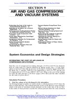
pump characteristic curves for the tentatively selected floor-mounted units are
shown in Fig. 1; one operating pump and one standby pump, each 0.75 hp (0.56

kW) are being considered. Can energy be conserved, and how much, with some
other pumping arrangement?
Calculation Procedure:
1. Plot the characteristic curves for the pumps being considered
Figure 2 shows the characteristic curves for the proposed pumps. Point 1 in Fig. 1
is the proposed operating head and flow rate. An alternative pump choice is shown
at Point 2 in Fig. 1. If two of the smaller pumps requiring only 0.25 hp (0.19 kW)
each are placed in series, they can generate the required 26-ft (7.9-m) head.
2. Analyze the proposed pumps
To analyze properly the proposal, a new set of curves, Fig. 2, is required. For the
proposed series pumping application, it is necessary to establish a seriesed pump
curve. This is a plot of the head and flow rate (capacity) which exists when both
pumps are running in series. To construct this curve, double the single-pump head
values at any given flow rate.
Next, to determine accurately the flow a single pump can deliver, plot the
system-head curve using the same method fully described in the previous calcula-
tion procedure. This curve is also plotted on Fig. 2.
Plot the point of operation for each pump on the seriesed curve, Fig. 2. The
point of operation of each pump is on the single-pump curve when both pumps are
operating. Each pump supplies half the total required head.
When a single pump is running, the point of operation will be at the intersection
of the system-head curve and the single-pump characteristic curve, Fig. 2. At this
point both the flow and the hp (kW) input of the single pump decrease. Series
pumping, Fig. 2, requires the input motor hp (kW) for both pumps; this is the point
of maximum power input.
3. Compute the possible savings
If the system requires a constant flow of 45 gal/min (2.84 L/ s) at 26-ft (7.9-m)
head the two-pump series installation saves (0.75 hp
Ϫ
2

ϫ
0.25 hp)
ϭ
0.25 hp
(0.19 kW) for every hour the pumps run. For every 1000 hours of operation, the
system saves 190 kWh. Since 2000 hours are generally equal to one shift of op-
eration per year, the saving is 380 kWh per shift per year.
If the load is frequently less than peak, one-pump operation delivers 32.5 gal/
min (2.1 L/ s). This value, which is some 72 percent of full load, corresponds to
doubling the saving.
Related Calculations. Series operation of pumps can be used in a variety of
designs for industrial, commercial, residential, chemical, power, marine, and similar
plants. A series connection of pumps is especially suitable when full-load demand
is small; i.e., just a few hours a week, month, or year. With such a demand, one
pump can serve the plant’s needs most of the time, thereby reducing the power bill.
When full-load operation is required, the second pump is started. If there is a need
for maintenance of the first pump, the second unit is available for service.
This procedure is the work of Jerome F. Mueller, P.E., of Mueller Engineering
Corp.
Downloaded from Digital Engineering Library @ McGraw-Hill (www.digitalengineeringlibrary.com)
Copyright © 2006 The McGraw-Hill Companies. All rights reserved.
Any use is subject to the Terms of Use as given at the website.
PUMPS AND PUMPING SYSTEMS
PUMPS AND PUMPING SYSTEMS
7.5
0
35
30
25
20

15
10
5
0
0 1020304050607080
0
2.5
5.0
7.5
10.0
12345
3/4 HP PUMP
(0.56 kW)
1/2 HP PUMP
(0.37 kW)
1/4 HP PUMP
(0.19 kW)
1/6 HP PUMP
(0.12 kW)
1
2
GPM
L/s
HEAD - FEET
Head, m
FIGURE 1 Pump characteristic curves for use in series installation.
PARALLEL PUMPING ECONOMICS
A system proposed for heating a 20,000-ft
2
(1858-m

2
) addition to an industrial plant
using hot-water heating requires a flow of 80 gal/ min (7.4 L/s) of 200
Њ
F (92.5
Њ
C)
water at a 20
Њ
F (36
Њ
C) temperature drop and a 13-ft (3.96-m) system head. The
Downloaded from Digital Engineering Library @ McGraw-Hill (www.digitalengineeringlibrary.com)
Copyright © 2006 The McGraw-Hill Companies. All rights reserved.
Any use is subject to the Terms of Use as given at the website.
PUMPS AND PUMPING SYSTEMS
7.6
PLANT AND FACILITIES ENGINEERING
0
35
30
25
20
15
10
5
0
0102030 4050607080
0
2.5

5.0
7.5
10.0
12 3 4 5
GPM
L/s
HEAD - FEET
Head, m
OPERATING POINT
OF EACH PUMP WHEN
BOTH ARE RUNNING
SINGLE PUMP
OPERATING POINT
SINGLE PUMP
CURVE
SYSTEM CURVE
SERIESED
PUMP CURVE
DESIGN
OPERATING
CONDITION
FIGURE 2 Seriesed-pump characteristic and system-head curves.
required system flow can be handled by two pumps, one an operating unit and one
a spare unit. Each pump will have an 0.5-hp (0.37-kW) drive motor. Could there
be any appreciable energy saving using some other arrangement? The system re-
quires 50 hours of constant pump operation and 40 hours of partial pump operation
per week.
Downloaded from Digital Engineering Library @ McGraw-Hill (www.digitalengineeringlibrary.com)
Copyright © 2006 The McGraw-Hill Companies. All rights reserved.
Any use is subject to the Terms of Use as given at the website.

PUMPS AND PUMPING SYSTEMS
PUMPS AND PUMPING SYSTEMS
7.7
010
5
25
20
15
10
5
0
0 20 40 60 80 100 120 140 160
9.0
7.5
6.0
4.5
3.0
1.5
0
1/2 HP PUMP (0.37 kW)
SYSTEM LOAD
1/4 HP PUMP
(0.10 kW)
GALLONS PER MINUTE
FEET OF HEAD
Head, m
L/s
FIGURE 3 Typical pump characteristic curves.
Calculation Procedure:
1. Plot characteristic curves for the proposed system

Figure 3 shows the proposed hot-water heating-pump selection for this industrial
building. Looking at the values of the pump head and capacity in Fig. 3, it can be
seen that if the peak load of 80 gal /min (7.4 L /s) were carried by two pumps, then
each would have to pump only 40 gal/min (3.7 L/s) in a parallel arrangement.
2. Plot a characteristic curve for the pumps in parallel
Construct the paralleled-pump curve by doubling the flow of a single pump at any
given head, using data from the pump manufacturer. At 13-ft head (3.96-m) one
pump produces 40 gal /min (3.7 L /s); two pumps 80 gal/min (7.4 L /s). The re-
sulting curve is shown in Fig. 4.
The load for this system could be divided among three, four, or more pumps, if
desired. To achieve the best results, the number of pumps chosen should be based
on achieving the proper head and capacity requirements in the system.
3. Construct a system-head curve
Based on the known flow rate, 80 gal/ min (7.4 L /s) at 13-ft (3.96-m) head, a
system-head curve can be constructed using the fact that pumping head varies as
the square of the change in flow, or Q
2
/Q
1
ϭ
H
2
/H
1
, where Q
1
ϭ
known design
flow, gal /min (L/s); Q
2

ϭ
selected flow, gal/min (L /s); H
1
ϭ
known design head,
ft (m); H
2
ϭ
resultant head related to selected flow rate, gal /min (L/s)
Figure 5 shows the plotted system-head curve. Once the system-head curve is
plotted, draw the single-pump curve from Fig. 3 on Fig. 5, and the parallelled-
pump curve from Fig. 4. Connect the different pertinent points of concern with
dashed lines, Fig. 5.
Downloaded from Digital Engineering Library @ McGraw-Hill (www.digitalengineeringlibrary.com)
Copyright © 2006 The McGraw-Hill Companies. All rights reserved.
Any use is subject to the Terms of Use as given at the website.
PUMPS AND PUMPING SYSTEMS
7.8
PLANT AND FACILITIES ENGINEERING
25
20
15
10
5
0
5010
L/s
9.0
7.5
6.0

4.5
3.0
1.5
0
Head, m
0 20 40 60 80 100 120 140 160
GALLONS PER MINUTE
ONE PUMP TWO PUMPS
Paralleled
FIGURE 4 Single- and dual-parallel pump characteristic curves.
25
20
15
10
5
0
9.0
7.5
6.0
4.5
3.0
1.5
0
5010
L/s
FEET OF HEAD
Head, m
0 20 40 60 80 100 120 140 160
TWO PUMPS
SINGLE PUMP

SYSTEM CURVE
GALLONS PER MINUTE
FIGURE 5 System-head curve for parallel pumping.
Downloaded from Digital Engineering Library @ McGraw-Hill (www.digitalengineeringlibrary.com)
Copyright © 2006 The McGraw-Hill Companies. All rights reserved.
Any use is subject to the Terms of Use as given at the website.
PUMPS AND PUMPING SYSTEMS
PUMPS AND PUMPING SYSTEMS
7.9
The point of crossing of the two-pump curve and the system-head curve is at
the required value of 80 gal/ min (7.4 L /s) and 13-ft (3.96-m) head because it was
so planned. But the point of crossing of the system-head curve and the single-pump
curve is of particular interest.
The single pump, instead of delivering 40 gal/min (7.4 L/s) at 13-ft (3.96-m)
head will deliver, as shown by the intersection of the curves in Fig. 5, 72 gal /min
(6.67 L/s) at 10-ft (3.05-m) head. Thus, the single pump can effectively be a
standby for 90 percent of the required capacity at a power input of 0.5 hp (0.37
kW). Much of the time in heating and air conditioning, and frequently in industrial
processes, the system load is 90 percent, or less.
4. Determine the single-pump horsepower input
In the installation here, the pumps are the inline type with non-overload motors.
For larger flow rates, the pumps chosen would be floor-mounted units providing a
variety of horsepower (kW) and flow curves. The horsepower (kW) for—say a 200-
gal/min (18.6 L/s) flow rate would be about half of a 400-gal/min (37.2 L /s) flow
rate.
If a pump were suddenly given a 300-gal/min (27.9 L/s) flow-rate demand at
its crossing point on a larger system-head curve, the hp required might be excessive.
Hence, the pump drive motor must be chosen carefully so that the power required
does not exceed the motor’s rating. The power input required by any pump can be
obtained from the pump characteristic curve for the unit being considered. Such

curves are available free of charge from the pump manufacturer.
The pump operating point is at the intersection of the pump characteristic curve
and the system-head curve in conformance with the first law of thermodynamics,
which states that the energy put into the system must exactly match the energy
used by the system. The intersection of the pump characteristic curve and the
system-head curve is the only point that fulfills this basic law.
There is no practical limit for pumps in parallel. Careful analysis of the system-
head curve versus the pump characteristic curves provided by the pump manufac-
turer will frequently reveal cases where the system load point may be beyond the
desired pump curve. The first cost of two or three smaller pumps is frequently no
greater than for one large pump. Hence, smaller pumps in parallel may be more
desirable than a single large pump, from both the economic and reliability stand-
points.
One frequently overlooked design consideration in piping for pumps is shown
in Fig. 6. This is the location of the check valve to prevent reverse-flow pumping.
Figure 6 shows the proper location for this simple valve.
5. Compute the energy saving possible
Since one pump can carry the fluid flow load about 90 percent of the time, and
this same percentage holds for the design conditions, the saving in energy is
0.9
ϫ
(0.5 kW
Ϫ
.25 kW)
ϫ
90 h per week
ϭ
20.25 kWh / week. (In this com-
putation we used the assumption that 1 hp
ϭ

1 kW.) The annual savings would be
52 weeks
ϫ
20.25 kW/week
ϭ
1053 kWh/yr. If electricity costs 5 cents per kWh,
the annual saving is $0.05
ϫ
1053
ϭ
$52.65/yr.
While a saving of some $51 per year may seem small, such a saving can become
much more if: (1) larger pumps using higher horsepower (kW) motors are used;
(2) several hundred pumps are used in the system; (3) the operating time is
longer—168 hours per week in some systems. If any, or all, these conditions prevail,
the savings can be substantial.
Downloaded from Digital Engineering Library @ McGraw-Hill (www.digitalengineeringlibrary.com)
Copyright © 2006 The McGraw-Hill Companies. All rights reserved.
Any use is subject to the Terms of Use as given at the website.
PUMPS AND PUMPING SYSTEMS
7.10
PLANT AND FACILITIES ENGINEERING
FIGURE 6 Check valve locations to prevent reverse flow.
Related Calculations. This procedure can be used for pumps in a variety of
applications: industrial, commercial, residential, medical, recreational, and similar
systems. When analyzing any system the designer should be careful to consider all
the available options so the best one is found.
This procedure is the work of Jerome F. Mueller, P.E., of Mueller Engineering
Corp.
USING CENTRIFUGAL PUMP SPECIFIC SPEED TO

SELECT DRIVER SPEED
A double-suction condenser circulator handling 20,000 gal /min (75,800 L/min) at
a total head of 60 ft (18.3 m) is to have a 15-ft (4.6-m) lift. What should be the
rpm of this pump to meet the capacity and head requirements?
Calculation Procedure:
1. Determine the specific speed of the pump
Use the Hydraulic Institute specific-speed chart, Fig. 7, page 7.11. Entering at 60
ft (18.3 m) head, project to the 15-ft suction lift curve. At the intersection, read the
specific speed of this double-suction pump as 4300.
2. Use the specific-speed equation to determine the pump operating rpm
Solve the specific-speed equation for the pump rpm. Or rpm
ϭ
N
s
ϫ
0.75 0.5
H /Q ,
where N
s
ϭ
specific speed of the pump, rpm, from Fig. 7; H
ϭ
total head on pump,
ft (m); Q
ϭ
pump flow rate, gal/min (L/min). Solving, rpm
ϭ
4300
ϫϭ
655.5 r/min. The next common electric motor rpm

0.75 0.5
60 /20,000
is 660; hence, we would choose a motor or turbine driver whose rpm does not
exceed 660.
Downloaded from Digital Engineering Library @ McGraw-Hill (www.digitalengineeringlibrary.com)
Copyright © 2006 The McGraw-Hill Companies. All rights reserved.
Any use is subject to the Terms of Use as given at the website.
PUMPS AND PUMPING SYSTEMS
PUMPS AND PUMPING SYSTEMS
7.11
FIGURE 7 Upper limits of specific speeds of single-stage, single- and double-suction
centrifugal pumps handling clear water at 85
Њ
F (29.4
Њ
C) at sea level. (Hydraulic Institute.)
The next lower induction-motor speed is 585 r/min. But we could buy a lower-
cost pump and motor if it could be run at the next higher full-load induction motor
speed of 700 r/min. The specific speed of such a pump would be: N
s
ϭ
[700
ϭ
4592. Referring to Fig. 7, the maximum suction lift with a
0.5 0.75
(20,000) ]/60
specific speed of 4592 is 13 ft (3.96 m) when the total head is 60 ft (18.3). If the
pump setting or location could be lowered 2 ft (0.6 m), the less expensive pump
and motor could be used, thereby saving on the investment cost.
Related Calculations. Use this general procedure to choose the driver and

pump rpm for centrifugal pumps used in boiler feed, industrial, marine, HVAC, and
similar applications. Note that the latest Hydraulic Institute curves should be used.
Downloaded from Digital Engineering Library @ McGraw-Hill (www.digitalengineeringlibrary.com)
Copyright © 2006 The McGraw-Hill Companies. All rights reserved.
Any use is subject to the Terms of Use as given at the website.
PUMPS AND PUMPING SYSTEMS
7.12
PLANT AND FACILITIES ENGINEERING
RANKING EQUIPMENT CRITICALITY TO COMPLY
WITH SAFETY AND ENVIRONMENTAL
REGULATIONS
Rank the criticality of a boiler feed pump operating at 250
Њ
F (121
Њ
C) and 100 lb /
in
2
(68.9 kPa) if its Mean Time Between Failures (MTBF) is 10 months, and vi-
bration is an important element in its safe operation. Use the National Fire Protec-
tion Association (NFPA) ratings of process chemicals for health, fire, and reactivity
hazards. Show how the criticality of the unit is developed.
Calculation Procedure:
1. Determine the Hazard Criticality Rating
(
HCR) of the equipment
Process industries of various types—chemical, petroleum, food, etc.—are giving
much attention to complying with new process safety regulations. These efforts
center on reducing hazards to people and the environment by ensuring the me-
chanical and electrical integrity of equipment.

To start a program, the first step is to evaluate the most critical equipment in a
plant or factory. To do so, the equipment is first ranked on some criteria, such as
the relative importance of each piece of equipment to the process or plant output.
The Hazard Criticality Rating (HCR) can be determined from a listing such as
that in Table 1. This tabulation contains the analysis guidelines for assessing the
process chemical hazard (PCH) and the Other Hazards (O). The ratings for such a
table of hazards should be based on the findings of an experienced team thoroughly
familiar with the process being evaluated. A good choice for such a task is the
plant’s Process Hazard Analysis (PHA) Group. Since a team’s familiarity with a
process is highest at the end of a PHA study, the best time for rating the criticality
of equipment is toward the end of such safety evaluations.
From Table 1, the NFPA rating, N, of process chemicals for Health, Fire, and
Reactivity, is N
ϭ
2, because this is the highest of such ratings for Health. The
Fire and Reactivity ratings are 0, 0, respectively, for a boiler feed pump because
there are no Fire or Reactivity exposures.
The Risk Reduction Factor (RF), from Table 1, is RF
ϭ
0, since there is the
potential for serious burns from the hot water handled by the boiler feed pump.
Then, the Process Chemical Hazard, PCH
ϭ
N
Ϫ
RF
ϭ
2
Ϫ
0

ϭ
2.
The rating of Other Hazards, O, Table 1, is O
ϭ
1, because of the high tem-
perature of the water. Thus, the Hazard Criticality Rating, HCR
ϭ
2, found from
the higher numerical value of PCH and O.
2. Determine the Process Criticality Rating, PCR, of the equipment
From Table 2, prepared by the PHA Group using the results of its study of the
equipment in the plant, PCR
ϭ
3. The reason for this is that the boiler feed pump
is critical for plant operation because its failure will result in reduced capacity.
3. Find the Process and Hazard Criticality Rating, PHCR
The alphanumeric PHC value is represented first by the alphabetic character for the
category. For example, Category A is the most critical, while Category D is the
least critical to plant operation. The first numeric portion represents the Hazard
Downloaded from Digital Engineering Library @ McGraw-Hill (www.digitalengineeringlibrary.com)
Copyright © 2006 The McGraw-Hill Companies. All rights reserved.
Any use is subject to the Terms of Use as given at the website.
PUMPS AND PUMPING SYSTEMS
PUMPS AND PUMPING SYSTEMS
7.13
TABLE 1
The Hazard Criticality Rating (HCR) is Determined in Three Steps*
Hazard Criticality Rating
1. Assess the Process Chemical Hazard (PCH) by:
●

Determining the NFPA ratings (N) of process chemicals for: Health, Fire, Reactivity
hazards
●
Selecting the highest value of N
●
Evaluating the potential for an emissions release (0 to 4):
High (RF
ϭ
0): Possible serious health, safety or environmental effects
Low (RF
ϭ
1): Minimal effects
None (RF
ϭ
4): No effects
●
Then, PCH
ϭ
N
Ϫ
RF. (Round off negative values to zero.)
2. Rate Other Hazards (O) with an arbitrary number (0 to 4) if they are:
●
Deadly (4), if:
Temperatures
Ͼ
1000
Њ
F
Pressures are extreme

Potential for release of regulated chemicals is high
Release causes possible serious health safety or environmental effects
Plant requires steam turbine trip mechanisms, fired-equipment shutdown systems,
or toxic- or combustible-gas detectors†
Failure of pollution control system results in environmental damage†
●
Extremely dangerous (3), if:
Equipment rotates at
Ͼ
5000 r/min
Temperatures
Ͼ
500
Њ
F
Plant requires process venting devices
Potential for release of regulated chemicals is low
Failure of pollution control system may result in environmental damage†
●
Hazardous (2), if:
Temperatures
Ͼ
300
Њ
F;
Extended failure of pollution control system may cause damage†
●
Slightly hazardous (1), if:
Equipment rotates at
Ͼ

3600 r/min
Temperatures
Ͼ
140
Њ
F or pressures
Ͼ
20 lb/in
2
(gage)
●
Not hazardous (0), if:
No hazards exist
3. Select the higher value of PCH and O as the Hazard Criticality Rating
*Chemical Engineering.
†Equipment with spares drop one category rating. A spare is an inline unit that can be immediately
serviced or be substituted by an alternative process option during the repair period.
Criticality Rating, HCR, while the second numeric part the Process Criticality Rat-
ing, PCR. These categories and ratings are a result of the work of the PHA Group.
From Table 3, the Process and Hazard Criticality Rating, PHCR
ϭ
B23. This is
based on the PCR
ϭ
3 and HCR
ϭ
2, found earlier.
4. Generate a criticality list by rating equipment using its alphanumeric
PHCR values
Each piece of equipment is categorized, in terms of its importance to the process,

as: Highest Priority, Category A; High Priority, Category B; Medium Priority, Cat-
egory C; Low Priority, Category D.
Downloaded from Digital Engineering Library @ McGraw-Hill (www.digitalengineeringlibrary.com)
Copyright © 2006 The McGraw-Hill Companies. All rights reserved.
Any use is subject to the Terms of Use as given at the website.
PUMPS AND PUMPING SYSTEMS
7.14
PLANT AND FACILITIES ENGINEERING
TABLE 2
Process Criticality Rating*
Process Criticality Rating
Essential
(4)
The equipment is essential if failure will result in shutdown of the unit,
unacceptable product quality, or severely reduced process yield
Critical
(3)
The equipment is critical if failure will result in greatly reduced capacity,
poor product quality, or moderately reduced process yield
Helpful
(2)
The equipment is helpful if failure will result in slightly reduced capacity,
product quality or reduced process yield
Not critical
(1)
The equipment is not critical if failure will have little or no process conse-
quences
*Chemical Engineering.
TABLE 3
The Process and Hazard Criticality Rating*

PHC Rankings
Process
Criticality
Rating
Hazard Criticality Rating
432 1 0
4 A44 A34 A24 A14 A04
3 A43 B33 B23 B13 B03
2 A42 A32 C22 C12 C02
1 A41 B31 C21 CD11 D01
Note: The alphanumeric PHC value is represented first by the
alphabetic character for the category (for example, category A is
the most critical while D is the least critical). The first numeric
portion represents the Hazard Criticality Rating, and the second
numeric part the Process Criticality Rating.
*Chemical Engineering.
Since the boiler feed pump is critical to the operation of the process, it is a
Category B, i.e., High Priority item in the process.
5. Determine the Criticality and Repetitive Equipment, CRE, value for this
equipment
This pump has an MTBF of 10 months. Therefore, from Table 4, CRE
ϭ
b1. Note
that the CRE value will vary with the PCHR and MTBF values for the equipment.
6. Determine equipment inspection frequency to ensure human and
environmental safety
From Table 5, this boiler feed pump requires vibration monitoring every 90 days.
With such monitoring it is unlikely that an excessive number of failures might
occur to this equipment.
7. Summarize criticality findings in spreadsheet form

When preparing for a PHCR evaluation, a spreadsheet, Table 6, listing critical
equipment, should be prepared. Then, as the various rankings are determined, they
can be entered in the spreadsheet where they are available for easy reference.
Downloaded from Digital Engineering Library @ McGraw-Hill (www.digitalengineeringlibrary.com)
Copyright © 2006 The McGraw-Hill Companies. All rights reserved.
Any use is subject to the Terms of Use as given at the website.
PUMPS AND PUMPING SYSTEMS
PUMPS AND PUMPING SYSTEMS
7.15
TABLE 4
The Criticality and Repetitive
Equipment Values*
CRE Values
PHCR
Mean time between
failures, months
0–6 6–12 12–24
Ͼ
24
Aa1a2a3a4
Ba2b1b2b3
Ca3b2c1c2
Da4b3c2d1
*Chemical Engineering.
TABLE 5
Predictive Maintenance
Frequencies for Rotating Equipment
Based on Their CRE Values*
Maintenance cycles
CRE

Frequency, days
7 30 90 360
a1, a2 VM LT
a3, a4 VM LT
b1, b3 VM
c1, d1 VM
VM: Vibration monitoring.
LT: Lubrication sampling and testing.
*Chemical Engineering.
TABLE 6
Typical Spreadsheet for Ranking Equipment Criticality*
Spreadsheet for calculating equipment PHCRS
Equipment
number
Equipment
description
NFPA rating
H F R RF PCH Other HCR PCR PHCR
TKO Tank 4 4 0 0 4 0 4 4 A44
TKO Tank 4 4 0 1 3 3 3 4 A34
PU1BFW Pump 2 0 0 0 2 1 2 3 B23
*Chemical Engineering.
Enter the PCH, Other, HCR, PCR, and PHCR values in the spreadsheet, as
shown. These data are now available for reference by anyone needing the infor-
mation.
Related Calculations. The procedure presented here can be applied to all types
of equipment used in a facility—fixed, rotating, and instrumentation. Once all the
equipment is ranked by criticality, priority lists can be generated. These lists can
Downloaded from Digital Engineering Library @ McGraw-Hill (www.digitalengineeringlibrary.com)
Copyright © 2006 The McGraw-Hill Companies. All rights reserved.

Any use is subject to the Terms of Use as given at the website.
PUMPS AND PUMPING SYSTEMS
7.16
PLANT AND FACILITIES ENGINEERING
then be used to ensure the mechanical integrity of critical equipment by prioritizing
predictive and preventive maintenance programs, inventories of critical spare parts,
and maintenance work orders in case of plant upsets.
In any plant, the hazards posed by different operating units are first ranked and
prioritized based on a PHA. These rankings are then used to determine the order
in which the hazards need to be addressed. When the PHAs approach completion,
team members evaluate the equipment in each operating unit using the PHCR sys-
tem.
The procedure presented here can be used in any plant concerned with human
and environmental safety. Today, this represents every plant, whether conventional
or automated. Industries in which this procedure finds active use include chemical,
petroleum, textile, food, power, automobile, aircraft, military, and general manu-
facturing.
This procedure is the work of V. Anthony Ciliberti, Maintenance Engineer, The
Lubrizol Corp., as reported in Chemical Engineering magazine.
Pump Affinity Laws, Operating Speed,
and Head
SIMILARITY OR AFFINITY LAWS FOR
CENTRIFUGAL PUMPS
A centrifugal pump designed for a 1800-r /min operation and a head of 200 ft (60.9
m) has a capacity of 3000 gal/min (189.3 L/ s) with a power input of 175 hp (130.6
kW). What effect will a speed reduction to 1200 r /min have on the head, capacity,
and power input of the pump? What will be the change in these variables if the
impeller diameter is reduced from 12 to 10 in (304.8 to 254 mm) while the speed
is held constant at 1800 r/min?
Calculation Procedure:

1. Compute the effect of a change in pump speed
For any centrifugal pump in which the effects of fluid viscosity are negligible, or
are neglected, the similarity or affinity laws can be used to determine the effect of
a speed, power, or head change. For a constant impeller diameter, the laws are
Q
1
/Q
2
ϭ
N
1
/N
2
; H
1
/H
2
ϭ
(N
1
/N
2
)
2
; P
1
/P
2
ϭ
(N

1
/N
2
)
3
. For a constant speed, Q
1
/
Q
2
ϭ
D
1
/D
2
; H
1
/H
2
ϭ
(D
1
/D
2
)
2
; P
1
/P
2

ϭ
(D
1
/D
2
)
3
. In both sets of laws,
Q
ϭ
capacity, gal / min; N
ϭ
impeller rpm; D
ϭ
impeller diameter, in; H
ϭ
total
head, ft of liquid; P
ϭ
bhp input. The subscripts 1 and 2 refer to the initial and
changed conditions, respectively.
For this pump, with a constant impeller diameter, Q
1
/Q
2
ϭ
N
1
/N
2

; 3000 /
Q
2
ϭ
1800/1200; Q
2
ϭ
2000 gal / min (126.2 L /s). And, H
1
/H
2
ϭ
(N
1
/
N
2
)
2
ϭ
200/ H
2
ϭ
(1800/1200)
2
; H
2
ϭ
88.9 ft (27.1 m). Also, P
1

/P
2
ϭ
(N
1
/
N
2
)
3
ϭ
175/ P
2
ϭ
(1800/1200)
3
; P
2
ϭ
51.8 bhp (38.6 kW).
Downloaded from Digital Engineering Library @ McGraw-Hill (www.digitalengineeringlibrary.com)
Copyright © 2006 The McGraw-Hill Companies. All rights reserved.
Any use is subject to the Terms of Use as given at the website.
PUMPS AND PUMPING SYSTEMS
PUMPS AND PUMPING SYSTEMS
7.17
2. Compute the effect of a change in impeller diameter
With the speed constant, use the second set of laws. Or, for this pump, Q
1
/

Q
2
ϭ
D
1
/D
2
; 3000/ Q
2
ϭ
12
⁄
10
; Q
2
ϭ
2500 gal/ min (157.7 L /s). And H
1
/
H
2
ϭ
(D
1
/D
2
)
2
; 200/H
2

ϭ
(
12
⁄
10
)
2
; H
2
ϭ
138.8 ft (42.3 m). Also, P
1
/P
2
ϭ
(D
1
/
D
2
)
3
; 175/P
2
ϭ
(
12
⁄
10
)

3
; P
2
ϭ
101.2 bhp (75.5 kW).
Related Calculations. Use the similarity laws to extend or change the data
obtained from centrifugal pump characteristic curves. These laws are also useful in
field calculations when the pump head, capacity, speed, or impeller diameter is
changed.
The similarity laws are most accurate when the efficiency of the pump remains
nearly constant. Results obtained when the laws are applied to a pump having a
constant impeller diameter are somewhat more accurate than for a pump at constant
speed with a changed impeller diameter. The latter laws are more accurate when
applied to pumps having a low specific speed.
If the similarity laws are applied to a pump whose impeller diameter is increased,
be certain to consider the effect of the higher velocity in the pump suction line.
Use the similarity laws for any liquid whose viscosity remains constant during
passage through the pump. However, the accuracy of the similarity laws decreases
as the liquid viscosity increases.
SIMILARITY OR AFFINITY LAWS IN
CENTRIFUGAL PUMP SELECTION
A test-model pump delivers, at its best efficiency point, 500 gal /min (31.6 L /s) at
a 350-ft (106.7-m) head with a required net positive suction head (NPSH) of 10 ft
(3 m) a power input of 55 hp (41 kW) at 3500 r /min, when a 10.5-in (266.7-mm)
diameter impeller is used. Determine the performance of the model at 1750 r/min.
What is the performance of a full-scale prototype pump with a 20-in (50.4-cm)
impeller operating at 1170 r/min? What are the specific speeds and the suction
specific speeds of the test-model and prototype pumps?
Calculation Procedure:
1. Compute the pump performance at the new speed

The similarity or affinity laws can be stated in general terms, with subscripts p and
m for prototype and model, respectively, as Q
p
ϭ
H
p
ϭ
322
KNQ ; KKH;
dnm d n m
NPSH
p
ϭ
P
p
ϭ
where K
d
ϭ
size factor
ϭ
prototype
22 5 5
KKNPSH ; KKP,
2 nm dnm
dimension/model dimension. The usual dimension used for the size factor is the
impeller diameter. Both dimensions should be in the same units of measure. Also,
K
n
ϭ

(prototype speed, r/min)/(model speed, r/min). Other symbols are the same
as in the previous calculation procedure.
When the model speed is reduced from 3500 to 1750 r/ min, the pump dimen-
sions remain the same and K
d
ϭ
1.0; K
n
ϭ
1750/3500
ϭ
0.5. Then Q
ϭ
(1.0)(0.5)(500)
ϭ
250 r / min; H
ϭ
(1.0)
2
(0.5)
2
(350)
ϭ
87.5 ft (26.7 m); NPSH
ϭ
(1.0)
2
(0.5)
2
(10)

ϭ
2.5 ft (0.76 m); P
ϭ
(1.0)
5
(0.5)
3
(55)
ϭ
6.9 hp (5.2 kW). In this
computation, the subscripts were omitted from the equations because the same
pump, the test model, was being considered.
Downloaded from Digital Engineering Library @ McGraw-Hill (www.digitalengineeringlibrary.com)
Copyright © 2006 The McGraw-Hill Companies. All rights reserved.
Any use is subject to the Terms of Use as given at the website.
PUMPS AND PUMPING SYSTEMS
7.18
PLANT AND FACILITIES ENGINEERING
2. Compute performance of the prototype pump
First, K
d
and K
n
must be found: K
d
ϭ
20/10.5
ϭ
1.905; K
n

ϭ
1170/3500
ϭ
0.335.
Then Q
p
ϭ
(1.905)
3
(0.335)(500)
ϭ
1158 gal/min (73.1 L/ s); H
p
ϭ
(1.905)
2
(0.335)
2
(350)
ϭ
142.5 ft (43.4 m); NPSH
p
ϭ
(1.905)
2
(0.335)
2
(10)
ϭ
4.06

ft (1.24 m); P
p
ϭ
(1.905)
5
(0.335)
3
(55)
ϭ
51.8 hp (38.6 kW).
3. Compute the specific speed and suction specific speed
The specific speed or, as Horwitz
1
says, ‘‘more correctly, discharge specific speed,’’
is N
s
ϭ
N while the suction specific speed S
ϭ
0.5 0.75 0.5 0.75
(Q)/(H), N(Q) /(NPSH) ,
where all values are taken at the best efficiency point of the pump.
For the model, N
s
ϭϭ
965; S
ϭ
0.5 0.75 0.5
3500(500) /(350) 3500(500) /
ϭ

13,900. For the prototype, N
s
ϭϭ
965;
0.75 0.5 0.75
(10) 1170(1158) /(142.5)
S
ϭϭ
13,900. The specific speed and suction specific
0.5 0.75
1170(1156) /(4.06)
speed of the model and prototype are equal because these units are geometrically
similar or homologous pumps and both speeds are mathematically derived from the
similarity laws.
Related Calculations. Use the procedure given here for any type of centrifugal
pump where the similarity laws apply. When the term model is used, it can apply
to a production test pump or to a standard unit ready for installation. The procedure
presented here is the work of R. P. Horwitz, as reported in Power magazine.
1
SPECIFIC SPEED CONSIDERATIONS IN
CENTRIFUGAL PUMP SELECTION
What is the upper limit of specific speed and capacity of a 1750-r / min single-stage
double-suction centrifugal pump having a shaft that passes through the impeller
eye if it handles clear water at 85
Њ
F (29.4
Њ
C) at sea level at a total head of 280 ft
(85.3 m) with a 10-ft (3-m) suction lift? What is the efficiency of the pump and
its approximate impeller shape?

Calculation Procedure:
1. Determine the upper limit of specific speed
Use the Hydraulic Institute upper specific-speed curve, Fig. 7, for centrifugal pumps
or a similar curve, Fig. 8, for mixed- and axial-flow pumps. Enter Fig. 7 at the
bottom at 280-ft (85.3-m) total head, and project vertically upward until the 10-ft
(3-m) suction-lift curve is intersected. From here, project horizontally to the right
to read the specific speed N
S
ϭ
2000. Figure 8 is used in a similar manner.
2. Compute the maximum pump capacity
For any centrifugal, mixed- or axial-flow pump, N
S
ϭ
where
0.5 0.75
(gpm)(rpm )/H ,
t
H
t
ϭ
total head on the pump, ft of liquid. Solving for the maximum capacity, we
get gpm
ϭ
/rpm)
2
ϭ
/1750)
2
ϭ

6040 gal /min (381.1
0.75 0.75
(NH (2000
ϫ
280
St
L/s).
1
R. P. Horwitz, ‘‘Affinity Laws and Specific Speed Can Simplify Centrifugal Pump Selection,’’ Power,
November 1964.
Downloaded from Digital Engineering Library @ McGraw-Hill (www.digitalengineeringlibrary.com)
Copyright © 2006 The McGraw-Hill Companies. All rights reserved.
Any use is subject to the Terms of Use as given at the website.
PUMPS AND PUMPING SYSTEMS
PUMPS AND PUMPING SYSTEMS
7.19
FIGURE 8 Upper limits of specific speeds of single-suction mixed-flow and axial-flow pumps.
(Hydraulic Institute.)
3. Determine the pump efficiency and impeller shape
Figure 9 shows the general relation between impeller shape, specific speed, pump
capacity, efficiency, and characteristic curves. At N
S
ϭ
2000, efficiency
ϭ
87 per-
cent. The impeller, as shown in Fig. 9, is moderately short and has a relatively
large discharge area. A cross section of the impeller appears directly under the
N
S

ϭ
2000 ordinate.
Related Calculations. Use the method given here for any type of pump whose
variables are included in the Hydraulic Institute curves, Figs. 7 and 8, and in similar
curves available from the same source. Operating specific speed, computed as
above, is sometimes plotted on the performance curve of a centrifugal pump so that
the characteristics of the unit can be better understood. Type specific speed is the
operating specific speed giving maximum efficiency for a given pump and is a
number used to identify a pump. Specific speed is important in cavitation and
suction-lift studies. The Hydraulic Institute curves, Figs. 7 and 8, give upper limits
of speed, head, capacity and suction lift for cavitation-free operation. When making
actual pump analyses, be certain to use the curves (Figs. 7 and 8) in the latest
edition of the Standards of the Hydraulic Institute.
SELECTING THE BEST OPERATING SPEED FOR A
CENTRIFUGAL PUMP
A single-suction centrifugal pump is driven by a 60-Hz ac motor. The pump delivers
10,000 gal/ min (630.9 L /s) of water at a 100-ft (30.5-m) head. The available net
Downloaded from Digital Engineering Library @ McGraw-Hill (www.digitalengineeringlibrary.com)
Copyright © 2006 The McGraw-Hill Companies. All rights reserved.
Any use is subject to the Terms of Use as given at the website.
PUMPS AND PUMPING SYSTEMS
7.20
PLANT AND FACILITIES ENGINEERING
FIGURE 9 Approximate relative impeller shapes and efficiency variations for various specific
speeds of centrifugal pumps. (Worthington Corporation.)
positive suction head
ϭ
32 ft (9.7 m) of water. What is the best operating speed
for this pump if the pump operates at its best efficiency point?
Calculation Procedure:

1. Determine the specific speed and suction specific speed
Ac motors can operate at a variety of speeds, depending on the number of poles.
Assume that the motor driving this pump might operate at 870, 1160, 1750, or
3500 r/min. Compute the specific speed N
S
ϭ
N
ϭ
0.5 0.75
(Q)/(H)
ϭ
3.14N and the suction specific speed S
ϭ
0.5 0.75 0.5
N(10,000) /(100) N(Q)/
ϭϭ
7.43N for each of the assumed speeds. Tabu-
0.75 0.5 0.75
(NPSH) N(10,000) /(32)
late the results as follows:
Downloaded from Digital Engineering Library @ McGraw-Hill (www.digitalengineeringlibrary.com)
Copyright © 2006 The McGraw-Hill Companies. All rights reserved.
Any use is subject to the Terms of Use as given at the website.
PUMPS AND PUMPING SYSTEMS
PUMPS AND PUMPING SYSTEMS
7.21
TABLE 7
Pump Types Listed by Specific
Speed*
TABLE 8

Suction Specific-Speed Ratings*
2. Choose the best speed for the pump
Analyze the specific speed and suction specific speed at each of the various oper-
ating speeds, using the data in Tables 7 and 8. These tables show that at 870 and
1160 r/min, the suction specific-speed rating is poor. At 1750 r/ min, the suction
specific-speed rating is excellent, and a turbine or mixed-flow type pump will be
suitable. Operation at 3500 r/min is unfeasible because a suction specific speed of
26,000 is beyond the range of conventional pumps.
Related Calculations. Use this procedure for any type of centrifugal pump
handling water for plant services, cooling, process, fire protection, and similar re-
quirements. This procedure is the work of R. P. Horwitz, Hydrodynamics Division,
Peerless Pump, FMC Corporation, as reported in Power magazine.
TOTAL HEAD ON A PUMP HANDLING
VAPOR-FREE LIQUID
Sketch three typical pump piping arrangements with static suction lift and sub-
merged, free, and varying discharge head. Prepare similar sketches for the same
pump with static suction head. Label the various heads. Compute the total head on
each pump if the elevations are as shown in Fig. 10 and the pump discharges a
maximum of 2000 gal/ min (126.2 L /s) of water through 8-in (203.2-mm) schedule
40 pipe. What hp is required to drive the pump? A swing check valve is used on
the pump suction line and a gate valve on the discharge line.
Calculation Procedure:
1. Sketch the possible piping arrangements
Figure 10 shows the six possible piping arrangements for the stated conditions of
the installation. Label the total static head, i.e., the vertical distance from the surface
Downloaded from Digital Engineering Library @ McGraw-Hill (www.digitalengineeringlibrary.com)
Copyright © 2006 The McGraw-Hill Companies. All rights reserved.
Any use is subject to the Terms of Use as given at the website.
PUMPS AND PUMPING SYSTEMS
7.22

PLANT AND FACILITIES ENGINEERING
FIGURE 10 Typical pump suction and discharge piping arrangements.
of the source of the liquid supply to the free surface of the liquid in the discharge
receiver, or to the point of free discharge from the discharge pipe. When both the
suction and discharge surfaces are open to the atmosphere, the total static head
equals the vertical difference in elevation. Use the free-surface elevations that cause
the maximum suction lift and discharge head, i.e., the lowest possible level in the
supply tank and the highest possible level in the discharge tank or pipe. When the
supply source is below the pump centerline, the vertical distance is called the static
suction lift; with the supply above the pump centerline, the vertical distance is
called static suction head. With variable static suction head, use the lowest liquid
level in the supply tank when computing total static head. Label the diagrams as
shown in Fig. 10.
2. Compute the total static head on the pump
The total static head H
ts
ft
ϭ
static suction lift, h
sl
ft
ϩ
static discharge head h
sd
ft,
where the pump has a suction lift, s in Fig. 10a, b, and c. In these installations,
Downloaded from Digital Engineering Library @ McGraw-Hill (www.digitalengineeringlibrary.com)
Copyright © 2006 The McGraw-Hill Companies. All rights reserved.
Any use is subject to the Terms of Use as given at the website.
PUMPS AND PUMPING SYSTEMS

PUMPS AND PUMPING SYSTEMS
7.23
H
ts
ϭ
10
ϩ
100
ϭ
110 ft (33.5 m). Note that the static discharge head is computed
between the pump centerline and the water level with an underwater discharge, Fig.
10a; to the pipe outlet with a free discharge, Fig. 10b; and to the maximum water
level in the discharge tank, Fig. 10c. When a pump is discharging into a closed
compression tank, the total discharge head equals the static discharge head plus the
head equivalent, ft of liquid, of the internal pressure in the tank, or 2.31
ϫ
tank
pressure, lb /in
2
.
Where the pump has a static suction head, as in Fig. 10d, e, and ƒ, the total
static head H
ts
ft
ϭ
h
sd
Ϫ
static suction head h
sh

ft. In these installations,
H
t
ϭ
100
Ϫ
15
ϭ
85 ft (25.9 m).
The total static head, as computed above, refers to the head on the pump without
liquid flow. To determine the total head on the pump, the friction losses in the
piping system during liquid flow must be also determined.
3. Compute the piping friction losses
Mark the length of each piece of straight pipe on the piping drawing. Thus, in Fig.
10a, the total length of straight pipe L
t
ft
ϭ
8
ϩ
10
ϩ
5
ϩ
102
ϩ
5
ϭ
130 ft (39.6
m), if we start at the suction tank and add each length until the discharge tank is

reached. To the total length of straight pipe must be added the equivalent length of
the pipe fittings. In Fig. 10a there are four long-radius elbows, one swing check
valve, and one globe valve. In addition, there is a minor head loss at the pipe inlet
and at the pipe outlet.
The equivalent length of one 8-in (203.2-mm) long-radius elbow is 14 ft (4.3
m) of pipe, from Table 9. Since the pipe contains four elbows, the total equivalent
length
ϭ
4(14)
ϭ
56 ft (17.1 m) of straight pipe. The open gate valve has an
equivalent resistance of 4.5 ft (1.4 m); and the open swing check valve has an
equivalent resistance of 53 ft (16.2 m).
The entrance loss h
e
ft, assuming a basket-type strainer is used at the suction-
pipe inlet, is h
e
ft
ϭ
K
v
2
/2g, where K
ϭ
a constant from Fig. 11;
v ϭ
liquid
velocity, ft/s; g
ϭ

32.2 ft/s
2
(980.67 cm/s
2
). The exit loss occurs when the liquid
passes through a sudden enlargement, as from a pipe to a tank. Where the area of
the tank is large, causing a final velocity that is zero, h
ex
ϭ v
2
/2g .
The velocity
v
ft/s in a pipe
ϭ
gpm /2.448d
2
. For this pipe,
v ϭ
2000/
[(2.448)(7.98)
2
]
ϭ
12.82 ft/ s (3.91 m/ s). Then h
e
ϭ
0.74(12.82)
2
/[2(32.2)]

ϭ
1.89
ft (0.58 m), and h
ex
ϭ
(12.82)
2
/[(2)(32.2)]
ϭ
2.56 ft (0.78 m). Hence, the total
length of the piping system in Fig. 10a is 130
ϩ
56
ϩ
4.5
ϩ
53
ϩ
1.89
ϩ
2.56
ϭ
247.95 ft (75.6 m), say 248 ft (75.6 m).
Use a suitable head-loss equation, or Table 10, to compute the head loss for the
pipe and fittings. Enter Table 10 at an 8-in (203.2-mm) pipe size, and project
horizontally across to 2000 gal/min (126.2 L /s) and read the head loss as 5.86 ft
of water per 100 ft (1.8 m/30.5 m) of pipe.
The total length of pipe and fittings computed above is 248 ft (75.6 m). Then
total friction-head loss with a 2000 gal /min (126.2-L/ s) flow is ft
ϭ

H
ƒ
(5.86)(248/100)
ϭ
14.53 ft (4.5 m).
4. Compute the total head on the pump
The total head on the pump H
t
ϭ
H
ts
ϩ
For the pump in Fig. 10a,H .
ƒ
H
t
ϭ
110
ϩ
14.53
ϭ
124.53 ft (37.95 m), say 125 ft (38.1 m). The total head on
the pump in Fig. 10b and c would be the same. Some engineers term the total head
on a pump the total dynamic head to distinguish between static head (no-flow
vertical head) and operating head (rated flow through the pump).
The total head on the pumps in Fig. 10d, c, and ƒ is computed in the same way
as described above, except that the total static head is less because the pump has
Downloaded from Digital Engineering Library @ McGraw-Hill (www.digitalengineeringlibrary.com)
Copyright © 2006 The McGraw-Hill Companies. All rights reserved.
Any use is subject to the Terms of Use as given at the website.

PUMPS AND PUMPING SYSTEMS
7.24
TABLE 9
Resistance of Fittings and Valves (length of straight pipe giving equivalent resistance)
Downloaded from Digital Engineering Library @ McGraw-Hill (www.digitalengineeringlibrary.com)
Copyright © 2006 The McGraw-Hill Companies. All rights reserved.
Any use is subject to the Terms of Use as given at the website.
PUMPS AND PUMPING SYSTEMS
PUMPS AND PUMPING SYSTEMS
7.25
FIGURE 11 Resistance coefficients of pipe fittings. To convert to SI in the equation
for h,
v
2
would be measured in m / s and feet would be changed to meters. The following
values would also be changed from inches to millimeters: 0.3 to 7.6, 0.5 to 12.7, 1 to
25.4, 2 to 50.8, 4 to 101.6, 6 to 152.4 10 to 254, and 20 to 508. (Hydraulic Institute.)
Downloaded from Digital Engineering Library @ McGraw-Hill (www.digitalengineeringlibrary.com)
Copyright © 2006 The McGraw-Hill Companies. All rights reserved.
Any use is subject to the Terms of Use as given at the website.
PUMPS AND PUMPING SYSTEMS