Tài liệu Handbook of Mechanical Engineering Calculations P8 doc

8.1
SECTION 8
PIPING AND FLUID FLOW
PRESSURE SURGE IN FLUID PIPING
SYSTEMS
8.2
Pressure Surge in a Piping System
From Rapid Valve Closure
8.2
Piping Pressure Surge with Different
Material and Fluid
8.5
Pressure Surge in Piping System with
Compound Pipeline
8.6
PIPE PROPERTIES, FLOW RATE, AND
PRESSURE DROP
8.8
Quick Calculation of Flow Rate and
Pressure Drop in Piping Systems
8.8
Fluid Head-Loss Approximations for
All Types of Piping
8.10
Pipe-Wall Thickness and Schedule
Number
8.11
Pipe-Wall Thickness Determination by
Piping Code Formula
8.12
Determining the Pressure Loss in

Steam Piping
8.15
Piping Warm-Up Condensate Load
8.18
Steam Trap Selection for Industrial
Applications
8.20
Selecting Heat Insulation for High-
Temperature Piping
8.27
Orifice Meter Selection for a Steam
Pipe
8.29
Selection of a Pressure-Regulating
Valve for Steam Service
8.30
Hydraulic Radius and Liquid Velocity
in Water Pipes
8.33
Friction-Head Loss in Water Piping of
Various Materials
8.33
Chart and Tabular Determination of
Friction Head
8.36
Relative Carrying Capacity of Pipes
8.39
Pressure-Reducing Valve Selection for
Water Piping
8.41

Sizing a Water Meter
8.42
Equivalent Length of a Complex
Series Pipeline
8.43
Equivalent Length of a Parallel Piping
System
8.44
Maximum Allowable Height for a
Liquid Siphon
8.45
Water-Hammer Effects in Liquid
Pipelines
8.47
Specific Gravity and Viscosity of
Liquids
8.47
Pressure Loss in Piping Having
Laminar Flow
8.48
Determining the Pressure Loss in Oil
Pipes
8.49
Flow Rate and Pressure Loss in
Compressed-Air and Gas Piping
8.56
Flow Rate and Pressure Loss in Gas
Pipelines
8.57
Selecting Hangers for Pipes at

Elevated Temperatures
8.58
Hanger Spacing and Pipe Slope for an
Allowable Stress
8.66
Effect of Cold Spring on Pipe Anchor
Forces and Stresses
8.67
Reacting Forces and Bending Stress
in Single-Plane Pipe Bend
8.68
Reacting Forces and Bending Stress
in a Two-Plane Pipe Bend
8.75
Reacting Forces and Bending Stress
in a Three-Plane Pipe Bend
8.77
Anchor Force, Stress, and Deflection
of Expansion Bends
8.79
Slip-Type Expansion Joint Selection
and Application
8.80
Corrugated Expansion Joint Selection
and Application
8.84
Design of Steam Transmission Piping
8.88
Steam Desuperheater Analysis
8.98

Steam Accumulator Selection and
Sizing
8.100
Selecting Plastic Piping for Industrial
Use
8.102
Analyzing Plastic Piping and Lining
for Tanks, Pumps and Other
Components for Specific
Applications
8.104
Downloaded from Digital Engineering Library @ McGraw-Hill (www.digitalengineeringlibrary.com)
Copyright © 2006 The McGraw-Hill Companies. All rights reserved.
Any use is subject to the Terms of Use as given at the website.
Source: HANDBOOK OF MECHANICAL ENGINEERING CALCULATIONS
8.2
PLANT AND FACILITIES ENGINEERING
Friction Loss in Pipes Handling Solids
in Suspension
8.111
Desuperheater Water Spray Quantity
8.112
Sizing Condensate Return Lines for
Optimum Flow Conditions
8.114
Estimating Cost of Steam Leaks from
Piping and Pressure Vessels
8.116
Quick Sizing of Restrictive Orifices in
Piping

8.117
Steam Tracing a Vessel Bottom to
Keep Its Contents Fluid
8.118
Designing Steam-Transmission Lines
Without Steam Traps
8.119
Line Sizing for Flashing Steam
Condensate
8.124
Determining the Friction Factor for
Flow of Bingham Plastics
8.127
Time Needed to Empty a Storage
Vessel with Dished Ends
8.130
Time Needed to Empty a Vessel
Without Dished Ends
8.133
Time Needed to Drain a Storage Tank
Through Attached Piping
8.134
Pressure Surge in Fluid Piping Systems
PRESSURE SURGE IN A PIPING SYSTEM FROM
RAPID VALVE CLOSURE
Oil, with a specific weight of 52 lb /ft
3
(832 kg /m
3
) and a bulk modulus of 250,000

lb/in
2
(1723 MPa), flows at the rate of 40 gal /min (2.5 L/s) through stainless steel
pipe. The pipe is 40 ft (12.2 m) long, 1.5 in (38.1 mm) O.D., 1.402 in (35.6 mm)
I.D., 0.049 in (1.24 mm) wall thickness, and has a modulus of elasticity, E,of
29
ϫ
10
6
lb/in
2
(199.8 kPa
ϫ
10
6
). Normal static pressure immediately upstream
of the valve in the pipe is 500 lb/ in
2
(abs) (3445 kPa). When the flow of the oil
is reduced to zero in 0.015 s by closing a valve at the end of the pipe, what is: (a)
the velocity of the pressure wave; (b) the period of the pressure wave; (c) the
amplitude of the pressure wave; and (d) the maximum static pressure at the valve?
Calculation Procedure:
1. Find the velocity of the pressure wave when the valve is closed
(a) Use the equation
68.094
a
ϭ
͙
␥

[(1/K)
ϩ
(D/Et)]
where the symbols are as given in the notation below. Substituting,
68.094
a
ϭ
46
͙
52 [(1/25
ϫ
10 )
ϩ
(1.402/29
ϫ
10
ϫ
0.049]
ϭ
4228 ft/s (1288.7 m/s)
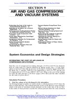
An alternative solution uses Fig. 1. With a D / t ratio
ϭ
1.402/0.049
ϭ
28.6 for
Downloaded from Digital Engineering Library @ McGraw-Hill (www.digitalengineeringlibrary.com)
Copyright © 2006 The McGraw-Hill Companies. All rights reserved.
Any use is subject to the Terms of Use as given at the website.
PIPING AND FLUID FLOW
PIPING AND FLUID FLOW

8.3
5,000
4,000
3,000
2,000
1524
1219
914
610
Bulk modulus K = 250,000 psi
Specific weight = 52 lb per cu ft
␥
S
t
a
i
n
l
e
s
s
s
t
e
e
l
p
i
p
e

,
E
=
2
9
x
1
0
6
p
s
i
C
o
p
p
e
r
p
i
p
e
,
E
=
1
7
x
1
0

6
p
s
i
A
l
u
m
i
n
u
m
p
i
p
e
,
E
=
1
0
.
7
x
1
0
6
p
s
i

0 14012010080604020
a, Velocity of pressure wave, ft per sec
Velocity, m/sec
D / t; I.D. of pipe / wall thickness
250,000 psi (1723 GPa) 300,000 psi (2.07 GPa)
52 lb/ft
3
(832 kg/m
3
) 62.42 lb/ft
3
(998.7 kg/m
3
)
29 ϫ 10
6
psi (199.8 GPa)
17 ϫ 10
6
psi (117.1 (GPa)
10.7 ϫ 10
6
psi (73.7 GPa)
FIGURE 1 Velocity of pressure wave in oil column in pipe of different diameter-to-
wall thickness ratios. (Product Engineering.)
stainless steel pipe, the velocity, a, of the pressure wave is 4228 ft/s (1288.7 m/
s).
2. Compute the time for the pressure wave to make one round trip in the pipe
b) The time for the pressure wave to make one round trip between the pipe ex-
tremities, or one interval, is: 2L / a

ϭ
2(40)/4228
ϭ
0.0189 s, and the period of the
pressure wave is: 2(2L/ a)
ϭ
2(0.0189)
ϭ
0.0378 s.
3. Calculate the pressure surge for rapid valve closure
c) Since the time of 01015 s for valve closure is less than the internal time
2L/a equal to 0.0189 s, the pressure surge can be computed from:
⌬
p
ϭ
␥
aV/144g
for rapid valve closure.
Downloaded from Digital Engineering Library @ McGraw-Hill (www.digitalengineeringlibrary.com)
Copyright © 2006 The McGraw-Hill Companies. All rights reserved.
Any use is subject to the Terms of Use as given at the website.
PIPING AND FLUID FLOW
8.4
PLANT AND FACILITIES ENGINEERING
The velocity of flow, V
ϭ
[(40)(231)(4)]/[(60)(
␲
)(1.402
2

)(12)] using the stan-
dard pipe flow relation, or V
ϭ
8.3 ft /s (2.53 m/ s).
Then, the amplitude of the pressure wave, using the equation above is:
52
ϫ
4228
ϫ
8.3
2
⌬
p
ϭϭ
393.5 lb/in (2711.2 kPa).
144
ϫ
32.2
4. Determine the resulting maximum static press in the pipe
d) The resulting maximum static pressure in the line, p
max
ϭ
p
ϩ ⌬
p
ϭ
500
ϩ
393.5
ϭ

893.5 lb /in
2
(abs) (6156.2 kPa).
Related Calculations. In an industrial hydraulic system, such as that used in
machine tools, hydraulic lifts, steering mechanisms, etc., when the velocity of a
flowing fluid is changed by opening or closing a valve, pressure surges result. The
amplitude of the pressure surge is a function of the rate of change in the velocity
of the mass of fluid. This procedure shows how to compute the amplitude of the
pressure surge with rapid valve closure.
The procedure is the work of Nils M. Sverdrup, Hydraulic Engineer, Aerojet-
General Corporation, as reported in Product Engineering magazine. SI values were
added by the handbook editor.
Notation
a
ϭ
velocity of pressure wave, ft/s (m /s)
a
E
ϭ
effective velocity of pressure wave, ft/s (m/s)
A
ϭ
cross-sectional area of pipe, in
2
(mm
2
)
A
o
ϭ

area of throttling orifice before closure, in
2
(mm
2
)
c
ϭ
velocity of sound, ft /s (m /s)
C
D
ϭ
coefficient of discharge
D
ϭ
inside diameter of pipe, in (mm)
E
ϭ
modulus of elasticity of pipe material, lb/ in
2
(kPa)
F
ϭ
force, lb (kg)
g
ϭ
gravitational acceleration, 32.2 ft /s
2
K
ϭ
bulk modulus of fluid medium, lb /in

2
(kPa)
L
ϭ
length of pipe, ft (m)
m
ϭ
mass, slugs
N
ϭ
T/(2L/ a )
ϭ
number of pressure wave intervals during time of valve clo-
sure
p
ϭ
normal static fluid pressure immediately upstream of valve when the fluid
velocity is V, lb/in
2
(absolute) (kPa)
⌬
p
ϭ
amplitude of pressure wave, lb/in
2
(kPa)
p
max
ϭ
maximum static pressure immediately upstream of valve, lb/ in

2
(absolute)
(kPa)
p
d
ϭ
static pressure immediately downstream of the valve, lb /in
2
(absolute)
(kPa)
Q
ϭ
volume rate of flow, ft
3
/s (m
3
/s)
t
ϭ
wall thickness of pipe, in (mm)
T
ϭ
time in which valve is closed, s
v ϭ
fluid volume, in
3
(mm
3
)
v

A
ϭ
air volume, in
3
(mm
3
)
V
ϭ
normal velocity of fluid flow in pipe with valve wide open, ft/ s (m/s)
V
E
ϭ
equivalent fluid velocity, ft / s (m/ s)
V
n
ϭ
velocity of fluid flow during interval n, ft/s (m/s)
Downloaded from Digital Engineering Library @ McGraw-Hill (www.digitalengineeringlibrary.com)
Copyright © 2006 The McGraw-Hill Companies. All rights reserved.
Any use is subject to the Terms of Use as given at the website.
PIPING AND FLUID FLOW
PIPING AND FLUID FLOW
8.5
W
ϭ
work, ft
⅐
lb (W)
␥

ϭ
specific weight, lb/ft
3
(kg/m
3
)
␾
n
ϭ
coefficient dependent upon the rate of change in orifice area and dis-
charge coefficient
␶
ϭ
period of oscillation of air cushion in a sealed chamber, s
PIPING PRESSURE SURGE WITH DIFFERENT
MATERIAL AND FLUID
(a) What would be the pressure rise in the previous procedure if the pipe were
aluminum instead of stainless steel? (b) What would be the pressure rise in the
system in the previous procedure if the flow medium were water having a bulk
modulus, K, of 300,000 lb/in
2
(2067 MPa) and a specific weight of 62.42 lb /ft
3
(998.7 kg /m
3
)?
Calculation Procedure:
1. Find the velocity of the pressure wave in the pipe
(a) From Fig. 2, for aluminum pipe having a D/t ratio of 28.6, the velocity of the
pressure wave is 3655 ft/s (1114.0 m/s). Alternatively, the velocity could be com-

puted as in step 1 in the previous procedure.
2. Compute the time for one interval of the pressure wave
As before, in the previous procedure, 2 L / a
ϭ
2 (40 /3655)
ϭ
0.02188 s.
3. Calculate the pressure rise in the pipe
Since the time of 0.015 s for the valve closure is less than the interval time of 2
L/a equal to 0.02188, the pressure rise can be computed from:
⌬
p
ϭ
␥
aV/144g
or,
52
ϫ
3655
ϫ
8.3
2
⌬
p
ϭϭ
340.2 lb/in (2343.98 kPa)
144
ϫ
32.2
4. Find the maximum static pressure in the line

Using the pressure-rise relation, p
max
ϭ
500
ϩ
340.2
ϭ
840.2 lb/in
2
(abs) (5788.97
kPa).
5. Determine the pressure rise for the different fluid
(b) For water, use Fig. 2 for stainless steel pipe having a D /t ratio of 28.6 to find
a
ϭ
4147 ft/s (1264 m /s). Alternatively, the velocity could be calculated as in step
1 of the previous procedure.
6. Compute the time for one internal of the pressure wave
Using 2 L/ a
ϭ
2 (40) /4147
ϭ
0.012929 s.
Downloaded from Digital Engineering Library @ McGraw-Hill (www.digitalengineeringlibrary.com)
Copyright © 2006 The McGraw-Hill Companies. All rights reserved.
Any use is subject to the Terms of Use as given at the website.
PIPING AND FLUID FLOW
8.6
PLANT AND FACILITIES ENGINEERING
5,000

4,000
3,000
2,000
1524
1219
914
610
a, Velocity of pressure wave, ft per sec
Velocity, m/sec
0 14012010080604020
D / t; I.D. of pipe / wall thickness
See Fig. 1 for SI values
Bulk modulus K = 250,000 psi
Specific weight = 52 lb per cu ft
␥
S
t
a
i
n
l
e
s
s
s
t
e
e
l
p

i
p
e
,
E
=
2
9
x
1
0
6
p
s
i
C
o
p
p
e
r
p
i
p
e
,
E
=
1
7

x
1
0
6
p
s
i
A
l
u
m
i
n
u
m
p
i
p
e
,
E
=
1
0
.
7
x
1
0
6

p
s
i
FIGURE 2 Velocity of pressure wave in water column in pipe of different diameter-to-
wall thickness ratios. (Product Engineering.)
7. Find the pressure rise and maximum static pressure in the line
Since the time of 0.015 s for valve closure is less than the interval time 2 L / a equal
to 0.01929 s, the pressure rise can be computed from
⌬
p
ϭ
␥
aV/144g
for rapid valve closure. Therefore, the pressure rise when the flow medium is water
is:
62.42
ϫ
4147
ϫ
8.3
2
⌬
p
ϭϭ
463.4 lb/in (3192.8 kPa)
144
ϫ
32.2
The maximum static pressure, p
max

ϭ
500
ϩ
463.4
ϭ
963.4 lb/ in
2
(abs) (6637.8
kPa).
Related Calculations. This procedure is the work of Nils M. Sverdrup, as
detailed in the previous procedure.
PRESSURE SURGE IN PIPING SYSTEM WITH
COMPOUND PIPELINE
A compound pipeline consisting of several stainless-steel pipes of different diam-
eters, Fig. 3, conveys 40 gal/min (2.5 L / s) of water. The length of each section of
Downloaded from Digital Engineering Library @ McGraw-Hill (www.digitalengineeringlibrary.com)
Copyright © 2006 The McGraw-Hill Companies. All rights reserved.
Any use is subject to the Terms of Use as given at the website.
PIPING AND FLUID FLOW
PIPING AND FLUID FLOW
8.7
FIGURE 3 Compound pipeline
consists of pipe sections having dif-
ferent diameters. (Product Engineer-
ing.)
pipe is: L
1
ϭ
25 ft (7.6 m); L
2

ϭ
15 ft (4.6 m); L
3
ϭ
10 ft (3.0 m); pipe wall
thickness in each section is 0.049 in (1.24 mm); inside diameter of each section of
pipe is D
1
ϭ
1.402 in (35.6 mm); D
2
ϭ
1.152 in (29.3 mm); D
3
ϭ
0.902 in (22.9
mm). What is the equivalent fluid velocity and the effective velocity of the pressure
wave on sudden valve closure?
Calculation Procedure:
1. Determine fluid velocity and pressure-wave velocity in the first pipe
D
1
/t
1
ratio of the first pipe
ϭ
1.402/0.049
ϭ
28.6. Then, the fluid velocity in the
pipe can be found from V

1
ϭ
0.4085(G
n
/(D
n
)
2
, where the symbols are as shown
below. Substituting, V
1
ϭ
0.4085(40)/(1.402)
2
ϭ
8.31 ft /s (2.53 m/ s).
Using these two computed values, enter Fig. 2 to find the velocity of the pressure
wave in pipe 1 as 4147 ft / s (1264 m/ s).
2. Find the fluid velocity and pressure-wave velocity in the second pipe
The D
2
/t
2
ratio for the second pipe
ϭ
1.152/0.049
ϭ
23.51. Using the same ve-
locity equation as in step 1, above V
2

ϭ
0.4085(40)/(1.152)
2
ϭ
12.31 ft /s (3.75
m/s).
Again, from Fig. 2, a
2
ϭ
4234 ft/ s (1290.5 m/s). Thus, there is an 87-ft/s (26.5-
m/s) velocity increase of the pressure wave between pipes 1 and 2.
3. Compute the fluid velocity and pressure-wave velocity in the third pipe
Using a similar procedure to that in steps 1 and 2 above, V
3
ϭ
20.1 ft /s (6.13 m /
s); s
3
ϭ
4326 ft /s (1318.6 m / s).
4. Find the equivalent fluid velocity and effective pressure-wave velocity for
the compound pipe
Use the equation
LV
ϩ
LV
ϩ ⅐⅐⅐ ϩ
L V
11 22 nn
V

ϭ
E
L
ϩ
L
ϩ ⅐⅐⅐ ϩ
L
12 n
to find the equivalent fluid velocity in the compound pipe. Substituting,
Downloaded from Digital Engineering Library @ McGraw-Hill (www.digitalengineeringlibrary.com)
Copyright © 2006 The McGraw-Hill Companies. All rights reserved.
Any use is subject to the Terms of Use as given at the website.
PIPING AND FLUID FLOW
8.8
PLANT AND FACILITIES ENGINEERING
25
ϫ
8.3
ϩ
15
ϫ
12.3
ϩ
10
ϫ
20.1
V
ϭ
E
25

ϩ
15
ϩ
10
ϭ
11.9 ft/s (3.63 m/s)
To find the effective velocity of the pressure wave, use the equation
L
ϩ
L
ϩ ⅐⅐⅐
L
12 n
a
ϭ
g
(L /a )
ϩ
(L /a )
ϩ ⅐⅐⅐ ϩ
(L /a )
11 22 nn
Substituting,
25
ϩ
15
ϩ
10
a
ϭ

g
(25/4147)
ϩ
(15/4234)
ϩ
(10/4326)
ϭ
4209 ft/s (1282.9 m/s)
Thus, equivalent fluid velocity and effective velocity of the pressure wave in the
compound pipe are both less than either velocity in the individual sections of the
pipe.
Related Calculations. Compound pipes find frequent application in industrial
hydraulic systems. The procedure given here is useful in determining the velocities
produced by sudden closure of a valve in the line.
L
1
, L
2
,...,L
n
ϭ
length of each section of pipe of constant diameter, ft (m)
a
1
, a
2
,...,a
n
ϭ
velocity of pressure wave in the respective pipe sections, ft /s

(m/s)
a
g
ϭ
effective velocity of the pressure wave, ft/s
V
1
, V
2
,..V
n
ϭ
velocity of fluid in the respective pipe sections, ft / s (m / s)
V
E
ϭ
equivalent fluid velocity, ft / s (m/ s)
G
n
ϭ
rate of flow in respective section, U.S. gal/ min (L/ s)
D
n
ϭ
inside diameter of respective pipe, in (mm)
The fluid velocity in an individual pipe is
2
V
ϭ
0.4085G /D

nnn
This procedure is the work of Nils M. Sverdrup, as detailed earlier.
Pipe Properties, Flow Rate, and
Pressure Drop
QUICK CALCULATION OF FLOW RATE AND
PRESSURE DROP IN PIPING SYSTEMS
A 3-in (76-mm) Schedule 40S pipe has a 300-gal / min (18.9-L/ s) water flow rate
with a pressure loss of 8 lb / in
2
(55.1 kPa)/100 ft (30.5 m). What would be the
flow rate in a 4-in (102-mm) Schedule 40S pipe with the same pressure loss? What
would be the pressure loss in a 4-in (102-mm) Schedule 40S pipe with the same
Downloaded from Digital Engineering Library @ McGraw-Hill (www.digitalengineeringlibrary.com)
Copyright © 2006 The McGraw-Hill Companies. All rights reserved.
Any use is subject to the Terms of Use as given at the website.
PIPING AND FLUID FLOW
PIPING AND FLUID FLOW
8.9
flow rate, 300 gal /min (18.9 L /s)? Determine the flow rate and pressure loss for a
6-in (152-mm) Schedule 40S pipe with the same pressure and flow conditions.
Calculation Procedure:
1. Determine the flow rate in the new pipe sizes
Flow rate in a pipe with a fixed pressure drop is proportional to the ratio of (new
pipe inside diameter / known pipe inside diameter)
2.4
. This ratio is defined as the
flow factor, F. To use this ratio, the exact inside pipe diameters, known and new,
must be used. Take the exact inside diameter from a table of pipe properties.
Thus, with a 3-in (76-mm) and a 4-in (102-mm) Schedule 40S pipe conveying
water at a pressure drop of 8 lb/ in

2
(55.1 kPa)/100 ft (30.5 m), the flow factor
F
ϭ
(4.026/3.068)
2.4
ϭ
1.91975. Then, the flow rate, FR, in the large 4-in (102-
mm) pipe with the 8 lb/in
2
(55.1 kPa) pressure drop/100 ft (30.5 m), will be, FR
ϭ
1.91975
ϫ
300
ϭ
575.9 gal /min (36.3 L / s).
For the 6-in (152-mm) pipe, the flow rate with the same pressure loss will be
(6.065/3.068)
2.4
ϫ
300
ϭ
1539.8 gal /min (97.2 L / s).
2. Compute the pressure drops in the new pipe sizes
The pressure drop in a known pipe size can be extrapolated to a new pipe size by
using a pressure factor, P, when the flow rate is held constant. For this condition,
P
ϭ
(known inside diameter of the pipe/ new inside diameter of the pipe)

4.8
.
For the first situation given above, P
ϭ
(3.068/4.026)
4.8
ϭ
0.27134. Then, the
pressure drop, PD
N
, in the new 4-in (102-mm) Schedule 40S pipe with a 300-gal/
min (18.9-L/s) flow will be PD
N
ϩ
P(PD
K
), where PD
K
ϭ
pressure drop in the
known pipe size. Substituting, PD
N
ϭ
0.27134(8)
ϭ
2.17 lb / in
2
/100 ft (14.9 kPa/
30.5 m).
For the 6-in (152-mm) pipe, using the same approach, PD

N
ϭ
(3.068/6.065)
4.8
(8)
ϭ
0.303 lb /in
2
/100 ft (2.1 kPa/30.5 m).
Related Calculations. The flow and pressure factors are valuable timesavers
in piping system design because they permit quick determination of new flow rates
or pressure drops with minimum time input. When working with a series of pipe-
size possibilities of the same Schedule Number, the designer can compute values
for F and P in advance and apply them quickly. Here is an example of such a
calculation for Schedule 40S piping of several sizes:
Nominal pipe size,
new/known
Flow factor,
F
Nominal pipe size,
known/new
Pressure
factor,
P
2/ 1 5.092 1/2 0.0386
3/ 2 2.58 2/ 3 0.150
4/ 3 1.919 3/4 0.271
6/ 4 2.674 4/6 0.1399
8/ 6 1.933 6/8 0.267
10/ 8 1.726 8/10 0.335

12/ 10 1.542 10/12 0.421
When computing such a listing, the actual inside diameter of the pipe, taken from
a table of pipe properties, must be used when calculating F or P.
The F and P values are useful when designing a variety of piping systems for
chemical, petroleum, power, cogeneration, marine, buildings (office, commercial,
Downloaded from Digital Engineering Library @ McGraw-Hill (www.digitalengineeringlibrary.com)
Copyright © 2006 The McGraw-Hill Companies. All rights reserved.
Any use is subject to the Terms of Use as given at the website.
PIPING AND FLUID FLOW
8.10
PLANT AND FACILITIES ENGINEERING
residential, industrial), and other plants. Both the F and P values can be used for
pipes conveying oil, water, chemicals, and other liquids. The F and P values are
not applicable to steam or gases.
Note that the ratio of pipe diameters is valid for any units of measurement—
inches, cm, mm—provided the same units are used consistently throughout the
calculation. The results obtained using the F and P values usually agree closely
with those obtained using exact flow or pressure-drop equations. Such accuracy is
generally acceptable in everyday engineering calculations.
While the pressure drop in piping conveying a liquid is inversely proportional
to the fifth power of the pipe diameter ratio, turbulent flow alters this to the value
of 4.8, according to W. L. Nelson, Technical Editor, The Oil and Gas Journal.
FLUID HEAD-LOSS APPROXIMATIONS FOR ALL
TYPES OF PIPING
Using the four rules for approximating head loss in pipes conveying fluid under
turbulent flow conditions with a Reynolds number greater than 2100, find: (a)A
4-in (101.6-mm) pipe discharges 100 gal/min (6.3 L /s); how much fluid would a
2-in (50.8-mm) pipe discharge under the same conditions? (b) A 4-in (101.6-mm)
pipe has 240 gal/min (15.1 L/s) flowing through it. What would be the friction
loss in a 3-in (76.2-mm) pipe conveying the same flow? (c) A flow of 10 gal /min

(6.3 L / s) produces 50 ft (15.2 m) of friction in a pipe. How much friction will a
flow of 200 gal/min (12.6 L/s) produce? (d) A 12-in (304.8-mm) diameter pipe
has a friction loss of 200 ft (60.9 m) / 1000 ft (304.8 M). What is the capacity of
this pipe?
Calculation Procedure:
1. Use the rule: At constant head, pipe capacity is proportional to d
2.5
(a) Applying the constant-head rule for both pipes: 4
2.5
ϭ
32.0; 2
2.5
ϭ
5.66. Then,
the pipe capacity
ϭ
(flow rate, gal / min or L/s)(new pipe size
2.5
)/(previous pipe
size
2.5
)
ϭ
(100)(5.66)/32
ϭ
17.69 gal /min (1.11 L / s).
Thus, using this rule you can approximate pipe capacity for a variety of con-
ditions where the head is constant. This approximation is valid for metal, plastic,
wood, concrete, and other piping materials.
2. Use the rule: At constant capacity, head is proportional to 1/d

5
(b) We have a 4-in (101.6-mm) pipe conveying 240 gal /min (15.1 L / s). If we
reduce the pipe size to 3 in (76.2 mm) the friction will be greater because the flow
area is smaller. The head loss
ϭ
(flow rate, gal /min or L/s)(larger pipe diameter
to the fifth power)/ (smaller pipe diameter to the fifth power). Or, head
ϭ
(240)(4
5
)/(3
5
)
ϭ
1011 ft /1000 ft of pipe (308.3 m / 304.8 m of pipe).
Again, using this rule you can quickly and easily find the friction in a different
size pipe when the capacity or flow rate remains constant. With the easy availability
of handheld calculators in the field and computers in the design office, the fifth
power of the diameter is easily found.
3. Use the rule: At constant diameter, head is proportional to gal / min
(
L/s
)
2
(c) We know that a flow of 100 gal/ min (6.3 L/s) produces 50-ft (15.2-m) friction,
h, in a pipe. The friction, with a new flow will be, h
ϭ
(friction, ft or m, at known
Downloaded from Digital Engineering Library @ McGraw-Hill (www.digitalengineeringlibrary.com)
Copyright © 2006 The McGraw-Hill Companies. All rights reserved.

Any use is subject to the Terms of Use as given at the website.
PIPING AND FLUID FLOW
PIPING AND FLUID FLOW
8.11
flow rate)(new flow rate, gal/ min or L/ s
2
)/(previous flow rate, gal / min or L /s
2
).
Or, h
ϭ
(50)(200
2
)/(100
2
)
ϭ
200 ft (60.9 m).
Knowing that friction will increase as we pump more fluid through a fixed-
diameter pipe, this rule can give us a fast determination of the new friction. You
can even do the square mentally and quickly determine the new friction in a matter
of moments.
4. Use the rule: At constant diameter, capacity is proportional to friction, h
0.5
(d) Here the diameter is 12 in (304.8 mm) and friction is 200 ft (60.9 m)/1000 ft
(304.8 m). From a pipe friction chart, the nearest friction head is 84 ft (25.6 m)
for a flow rate of 5000 gal /min (315.5 L/s). The new capacity, c
ϭ
(known ca-
pacity, gal/min or L/s)(known friction, ft or m

0.5
)/(actual friction, ft or m
0.5
). Or,
c
ϭ
5000(200
0.5
)/(84
0.5
)
ϭ
7714 gal /min (486.6 L /s).
As before, a simple calculation, the ratio of the square roots of the friction heads
times the capacity will quickly give the new flow rates.
Related Calculations. Similar laws for fans and pumps give quick estimates
of changed conditions. These laws are covered elsewhere in this handbook in the
sections on fans and pumps. Referring to them now will give a quick comparison
of the similarity of these sets of laws.
PIPE-WALL THICKNESS AND
SCHEDULE NUMBER
Determine the minimum wall thickness t
m
in (mm) and schedule number SN for a
branch steam pipe operating at 900
Њ
F (482.2
Њ
C) if the internal steam pressure is
1000 lb/ in

2
(abs) (6894 kPa). Use ANSA B31.1 Code for Pressure Piping and the
ASME Boiler and Pressure Vessel Code valves and equations where they apply.
Steam flow rate is 72,000 lb / h (32,400 kg / h).
Calculation Procedure:
1. Determine the required pipe diameter
When the length of pipe is not given or is as yet unknown, make a first approxi-
mation of the pipe diameter, using a suitable velocity for the fluid. Once the length
of the pipe is known, the pressure loss can be determined. If the pressure loss
exceeds a desirable value, the pipe diameter can be increased until the loss is within
an acceptable range.
Compute the pipe cross-sectional area a in
2
(cm
2
) from a
ϭ
2.4W
v
/V, where
W
ϭ
steam flow rate, lb/ h (kg/ h);
v ϭ
specific volume of the steam, ft
3
/lb (m
3
/
kg); V

ϭ
steam velocity, ft/ min (m/min). The only unknown in this equation, other
than the pipe area, is the steam velocity V. Use Table 1 to find a suitable steam
velocity for this branch line.
Table 1 shows that the recommended steam velocities for branch steam pipes
range from 6000 to 15,000 ft/min (1828 to 4572 m/min). Assume that a velocity
of 12,000 ft/min (3657.6 m /min) is used in this branch steam line. Then, by using
the steam table to find the specific volume of steam at 900
Њ
F (482.2
Њ
C) and 1000
lb/in
2
(abs) (6894 kPa), a
ϭ
2.4(72,000)(0.7604)/12,000
ϭ
10.98 in
2
(70.8 cm
2
).
The inside diameter of the pipe is then d
ϭ
2(a/
␲
)
0.5
ϭ

2(10.98/
␲
)
0.5
ϭ
3.74 in
(95.0 mm). Since pipe is not ordinarily made in this fractional internal diameter,
round it to the next larger size, or 4-in (101.6-mm) inside diameter.
Downloaded from Digital Engineering Library @ McGraw-Hill (www.digitalengineeringlibrary.com)
Copyright © 2006 The McGraw-Hill Companies. All rights reserved.
Any use is subject to the Terms of Use as given at the website.
PIPING AND FLUID FLOW
8.12
PLANT AND FACILITIES ENGINEERING
TABLE 1
Recommended Fluid Velocities in Piping
2. Determine the pipe schedule number
The ANSA Code for Pressure Piping, commonly called the Piping Code, defines
schedule number as SN
ϭ
1000 P
i
/S, where P
i
ϭ
internal pipe pressure, lb/in
2
(gage); S
ϭ
allowable stress in the pipe, lb/in

2
, from Piping Code. Table 2 shows
typical allowable stress values for pipe in power piping systems. For this pipe,
assuming that seamless ferritic alloy steel (1% Cr, 0.55% Mo) pipe is used with
the steam at 900
Њ
F (482
Њ
C), SN
ϭ
(1000)(1014.7)/13,100
ϭ
77.5. Since pipe is
not ordinarily made in this schedule number, use the next highest readily available
schedule number, or SN
ϭ
80. [Where large quantities of pipe are required, it is
sometimes economically wise to order pipe of the exact SN required. This is not
usually done for orders of less than 1000 ft (304.8 m) of pipe.]
3. Determine the pipe-wall thickness
Enter a tabulation of pipe properties, such as in Crocker and King—Piping Hand-
book, and find the wall thickness for 4-in (101.6-mm) SN 80 pipe as 0.337 in (8.56
mm).
Related Calculations. Use the method given here for any type of pipe—steam,
water, oil, gas, or air—in any service—power, refinery, process, commercial, etc.
Refer to the proper section of B31.1 Code for Pressure Piping when computing
the schedule number, because the allowable stress S varies for different types of
service.
The Piping Code contains an equation for determining the minimum required
pipe-wall thickness based on the pipe internal pressure, outside diameter, allowable

stress, a temperature coefficient, and an allowance for threading, mechanical
strength, and corrosion. This equation is seldom used in routine piping-system de-
sign. Instead, the schedule number as given here is preferred by most designers.
PIPE-WALL THICKNESS DETERMINATION BY
PIPING CODE FORMULA
Use the ANSA B31.1 Code for Pressure Piping wall-thickness equation to deter-
mine the required wall thickness for an 8.625-in (219.1-mm) OD ferritic steel plain-
Downloaded from Digital Engineering Library @ McGraw-Hill (www.digitalengineeringlibrary.com)
Copyright © 2006 The McGraw-Hill Companies. All rights reserved.
Any use is subject to the Terms of Use as given at the website.
PIPING AND FLUID FLOW
8.13
TABLE 2
Allowable Stresses (S Values) for Alloy-Steel Pipe in Power Piping Systems*
(Abstracted from ASME Power Boiler Code and Code for Pressure Piping, ASA B31.1)
Downloaded from Digital Engineering Library @ McGraw-Hill (www.digitalengineeringlibrary.com)
Copyright © 2006 The McGraw-Hill Companies. All rights reserved.
Any use is subject to the Terms of Use as given at the website.
PIPING AND FLUID FLOW
8.14
PLANT AND FACILITIES ENGINEERING
end pipe if the pipe is used in 900
Њ
F (482
Њ
C) 900-lb/in
2
(gage) (6205-kPa) steam
service.
Calculation Procedure:

1. Determine the constants for the thickness equation
Pipe-wall thickness to meet ANSA Code requirements for power service is com-
puted from t
m
ϭ
{DP/[2(S
ϩ
YP)]}
ϩ
C, where t
m
ϭ
minimum wall thickness, in;
D
ϭ
outside diameter of pipe, in; P
ϭ
internal pressure in pipe, lb/in
2
(gage);
S
ϭ
allowable stress in pipe material, lb /in
2
; Y
ϭ
temperature coefficient; C
ϭ
end-
condition factor, in.

Values of S, Y, and C are given in tables in the Code for Pressure Piping in the
section on Power Piping. Using values from the latest edition of the Code, we get
S
ϭ
12,500 lb/in
2
(86.2 MPa) for ferritic-steel pipe operating at 900
Њ
F (482
Њ
C);
Y
ϭ
0.40 at the same temperature; C
ϭ
0.065 in (1.65 mm) for plain-end steel
pipe.
2. Compute the minimum wall thickness
Substitute the given and Code values in the equation in step 1, or t
m
ϭ
[(8.625)(900)]/[2(12,500
ϩ
0.4
ϫ
900)]
ϩ
0.065
ϭ
0.367 in (9.32 mm).

Since pipe mills do not fabricate to precise wall thicknesses, a tolerance above
or below the computed wall thickness is required. An allowance must be made in
specifying the wall thickness found with this equation by increasing the thickness
by 12
1
⁄
2
percent. Thus, for this pipe, wall thickness
ϭ
0.367
ϩ
0.125(0.367)
ϭ
0.413 in (10.5 mm).
Refer to the Code to find the schedule number of the pipe. Schedule 60 8-in
(203-mm) pipe has a wall thickness of 0.406 in (10.31 mm), and schedule 80 has
a wall thickness of 0.500 in (12.7 mm). Since the required thickness of 0.413 in
(10.5 mm) is greater than schedule 60 but less than schedule 80, the higher schedule
number, 80, should be used.
3. Check the selected schedule number
From the previous calculation procedure, SN
ϭ
1000 P
i
/S. From this pipe,
SN
ϭ
1000(900)/12,500
ϭ
72. Since piping is normally fabricated for schedule

numbers 10, 20, 30, 40, 60, 80, 100, 120, 140, and 160, the next larger schedule
number higher than 72, that is 80, will be used. This agrees with the schedule
number found in step 2.
Related Calculations. Use this method in conjunction with the appropriate
Code equation to determine the wall thickness of pipe conveying air, gas, steam,
oil, water, alcohol, or any other similar fluids in any type of service. Be certain to
use the correct equation, which in some cases is simpler than that used here. Thus,
for lead pipe, t
n
ϭ
Pd/2S, where P
ϭ
safe working pressure of the pipe, lb /in
2
(gage); d
ϭ
inside diameter of pipe, in; other symbols as before.
When a pipe will operate at a temperature between two tabulated Code values,
find the allowable stress by interpolating between the tabulated temperature and
stress values. Thus, for a pipe operating at 680
Њ
F (360
Њ
C), find the allowable stress
at 650
Њ
F (343
Њ
C) [
ϭ

9500 lb/in
2
(65.5 MPa)] and 700
Њ
F (371
Њ
C) [
ϭ
9000 lb/in
2
(62.0 MPa)]. Interpolate thus: allowable stress at 680
Њ
F (360
Њ
C)
ϭ
[(700
Њ
F
Ϫ
680
Њ
F)/(700
Њ
F
Ϫ
650
Њ
F)](9500
Ϫ

9000)
ϩ
9000
ϭ
200
ϩ
9000
ϭ
9200 lb/ in
2
(63.4 MPa). The same result can be obtained by interpolating downward from 9500
Downloaded from Digital Engineering Library @ McGraw-Hill (www.digitalengineeringlibrary.com)
Copyright © 2006 The McGraw-Hill Companies. All rights reserved.
Any use is subject to the Terms of Use as given at the website.
PIPING AND FLUID FLOW
PIPING AND FLUID FLOW
8.15
lb/in
2
(65.5 MPa), or allowable stress at 680
Њ
F (360
Њ
C)
ϭ
9500
Ϫ
[(680
Ϫ
650)/

(700
Ϫ
650)](9500
Ϫ
9000)
ϭ
9200 lb /in
2
(63.4 MPa).
DETERMINING THE PRESSURE LOSS IN
STEAM PIPING
Use a suitable pressure-loss chart to determine the pressure loss in 510 ft (155.5
m) of 4-in (101.6-mm) flanged steel pipe containing two 90
Њ
elbows and four 45
Њ
bends. The schedule 40 piping conveys 13,000 lb /h (5850 kg /h) of 20-lb/in
2
(gage)
(275.8-kPa) 350
Њ
F (177
Њ
C) superheated steam. List other methods of determining
the pressure loss in steam piping.
Calculation Procedure:
1. Determine the equivalent length of the piping
The equivalent length of a pipe L
e
ft

ϭ
length of straight pipe, ft
ϩ
equivalent
length of fittings, ft. Using data from the Hydraulic Institute, Crocker and
King—Piping Handbook, earlier sections of this handbook, or Fig. 4, find the
equivalent length of a 90
Њ
4-in (101.6-mm) elbow as 10 ft (3 m) of straight pipe.
Likewise, the equivalent length of a 45
Њ
bend is 5 ft (1.5 m) of straight pipe.
Substituting in the above relation and using the straight lengths and the number of
fittings of each type, we get L
e
ϭ
510
ϩ
(2)(10)
ϩ
4(5)
ϭ
550 ft (167.6 m) of
straight pipe.
2. Compute the pressure loss, using a suitable chart
Figure 2 presents a typical pressure-loss chart for steam piping. Enter the chart at
the top left at the superheated steam temperature of 350
Њ
F (177
Њ

C), and project
vertically downward until the 40-lb /in
2
(gage) (275.8-kPa) superheated steam pres-
sure curve is intersected. From here, project horizontally to the right until the outer
border of the chart is intersected. Next, project through the steam flow rate, 13,000
lb/h (5900 kg/h) on scale B, Fig. 5, to the pivot scale C. From this point, project
through 4-in (101.6-mm) schedule 40 pipe on scale D, Fig. 5. Extend this line to
intersect the pressure-drop scale, and read the pressure loss as 7.25 lb/ in
2
(50
kPa)/100 ft (30.4 m) of pipe.
Since the equivalent length of this pipe is 550 ft (167.6 m), the total pressure
loss in the pipe is (550 / 100)(7.25)
ϭ
39.875 lb/ in
2
(274.9 kPa), say 40 lb/ in
2
(275.8 kPa).
3. List the other methods of computing pressure loss
Numerous pressure-loss equations have been developed to compute the pressure
drop in steam piping. Among the better known are those of Unwin, Fritzche, Spitz-
glass, Babcock, Guttermuth, and others. These equations are discussed in some
detail in Crocker and King—Piping Handbook and in the engineering data pub-
lished by valve and piping manufacturers.
Most piping designers use a chart to determine the pressure loss in steam piping
because a chart saves time and reduces the effort involved. Further, the accuracy
obtained is sufficient for all usual design practice.
Figure 3 is a popular flowchart for determining steam flow rate, pipe size, steam

pressure, or steam velocity in a given pipe. Using this chart, the designer can
Downloaded from Digital Engineering Library @ McGraw-Hill (www.digitalengineeringlibrary.com)
Copyright © 2006 The McGraw-Hill Companies. All rights reserved.
Any use is subject to the Terms of Use as given at the website.
PIPING AND FLUID FLOW
8.16
PLANT AND FACILITIES ENGINEERING
FIGURE 4 Equivalent length of pipe fittings and valves. (Crane Company.)
Downloaded from Digital Engineering Library @ McGraw-Hill (www.digitalengineeringlibrary.com)
Copyright © 2006 The McGraw-Hill Companies. All rights reserved.
Any use is subject to the Terms of Use as given at the website.
PIPING AND FLUID FLOW
8.17
FIGURE 5 Pressure loss in steam pipes based on the Fritzche formula. (Power.)
Downloaded from Digital Engineering Library @ McGraw-Hill (www.digitalengineeringlibrary.com)
Copyright © 2006 The McGraw-Hill Companies. All rights reserved.
Any use is subject to the Terms of Use as given at the website.
PIPING AND FLUID FLOW
8.18
PLANT AND FACILITIES ENGINEERING
determine any one of the four variables listed above when the other three are known.
In solving a problem on the chart in Fig. 6, use the steam-quantity lines to intersect
pipe sizes and the steam-pressure lines to intersect steam velocities. Here are two
typical applications of this chart.
Example. What size schedule 40 pipe is needed to deliver 8000 lb/ h (3600
kg/h) of 120-lb/ in
2
(gage) (827.3-kPa) steam at a velocity of 5000 ft /min (1524
m/min)?
Solution. Enter Fig. 6 at the upper left at a velocity of 5000 ft /min (1524 m/

min), and project along this velocity line until the 120-lb/in
2
(gage) (827.3-kPa)
pressure line is intersected. From this intersection, project horizontally until the
8000-lb/h (3600-kg/h) vertical line is intersected. Read the nearest pipe size as 4
in (101.6 mm) on the nearest pipe-diameter curve.
Example. What is the steam velocity in a 6-in (152.4-mm) pipe delivering
20,000 lb /h (9000 kg/h) of steam at 85 lb /in
2
(gage) (586 kPa)?
Solution. Enter the bottom of the chart, Fig. 6, at the flow rate of 20,000
lb/h (9000 kg/ h), and project vertically upward until the 6-in (152.4-mm) pipe
curve is intersected. From this point, project horizontally to the 85-lb/in
2
(gage)
(586-kPa) curve. At the intersection, read the velocity as 7350 ft / min (2240.3 m/
min).
Table 3 shows typical steam velocities for various industrial and commercial
applications. Use the given values as guides when sizing steam piping.
PIPING WARM-UP CONDENSATE LOAD
How much condensate is formed in 5 min during warm-up of 500 ft (152.4 m) of
6-in (152.4-mm) schedule 40 steel pipe conveying 215-lb/in
2
(abs) (1482.2-kPa)
saturated steam if the pipe is insulated with 2 in (50.8 mm) of 85 percent magnesia
and the minimum external temperature is 35
Њ
F (1.7
Њ
C)?

Calculation Procedure:
1. Compute the amount of condensate formed during pipe warm-up
For any pipe, the condensate formed during warm-up C
h
lb/h
ϭ
60(W
p
)(
⌬
t)(s)/
, where W
p
ϭ
total weight of pipe, lb;
⌬
t
ϭ
difference between final and initialhN
ƒg
temperature of the pipe,
Њ
F; s
ϭ
specific heat of pipe material, Btu/(lb
⅐ Њ
F);
ϭ
enthalpy of vaporization of the steam, Btu / lb; N
ϭ

warm-up time, min.h
ƒg
A table of pipe properties shows that this pipe weighs 18.974 lb/ft (28.1 kg/
m). The steam table shows that the temperature of 215-lb/in
2
(abs) (1482.2-kPa)
saturated steam is 387.89
Њ
F (197.7
Њ
C), say 388
Њ
F (197.8
Њ
C); the enthalpy
ϭ
837.4 Btu /lb (1947.8 kJ/kg). The specific heat of steel pipe s
ϭ
0.144 Btuh
ƒg
/(lb
⅐ Њ
F) [0.6 kJ / (kg
⅐ Њ
C)]. Then C
h
ϭ
60(500
ϫ
18.974)(388

Ϫ
35)(0.114)/
[(837.4)(5)]
ϭ
5470 lb /h (2461.5 kg /h).
2. Compute the radiation-loss condensate load
Condensate is also formed by radiation of heat from the pipe during warm-up and
while the pipe is operating. The warm-up condensate load decreases as the radiation
load increases, the peak occurring midway (2
1
⁄
2
min in this case) through the warm-
up period. For this reason, one-half the normal radiation load is added to the warm-
Downloaded from Digital Engineering Library @ McGraw-Hill (www.digitalengineeringlibrary.com)
Copyright © 2006 The McGraw-Hill Companies. All rights reserved.
Any use is subject to the Terms of Use as given at the website.
PIPING AND FLUID FLOW
8.19
FIGURE 6 Spitzglass chart for saturated steam flowing in schedule 40 pipe.
Downloaded from Digital Engineering Library @ McGraw-Hill (www.digitalengineeringlibrary.com)
Copyright © 2006 The McGraw-Hill Companies. All rights reserved.
Any use is subject to the Terms of Use as given at the website.
PIPING AND FLUID FLOW
8.20
PLANT AND FACILITIES ENGINEERING
TABLE 3
Steam Velocities Used in Pipe Design
up load. Where the radiation load is small, it is often disregarded. However, the
load must be computed before its magnitude can be determined.

For any pipe, C
r
ϭ
(L)(A)(
⌬
t)(H)/ , where L
ϭ
length of pipe, ft; A
ϭ
external
h
ƒg
area of pipe, ft
2
/ft of length; H
ϭ
heat loss through bare pipe or pipe insulation,
Btu/(ft
2
⅐
h
⅐ Њ
F), from the piping or insulation tables. This 6-in (152.4-mm) schedule
40 pipe has an external area A
ϭ
1.73 ft
2
/ft (0.53 m
2
/m) of length. The heat loss

through 2 in (50.8 mm) of 85 percent magnesia, from insulation tables, is H
ϭ
0.286 Btu/(ft
2
⅐
h
⅐ Њ
F) [1.62 W/(m
2
⅐ Њ
C)]. Then
C
r
ϭ
(500)
ϫ
(1.73)(388
Ϫ
35)(0.286)/837.4
ϭ
104.2 lb/ h (46.9 kg / h). Adding
half the radiation load to the warm-up load gives 5470
ϩ
52.1
ϭ
5522.1 lb / h
(2484.9 kg /h).
3. Apply a suitable safety factory to the condensate load
Trap manufacturers recommend a safety factor of 2 for traps installed between a
boiler and the end of a steam main; traps at the end of a long steam main or ahead

of pressure-regulating or shutoff valves usually have a safety factor of 3. With a
safety factor of 3 for this pipe, the steam trap should have a capacity of at least
3(5522.1)
ϭ
16,566.3 lb /h (7454.8 kg /h), say 17,000 lb / h (7650.0 kg/ h).
Related Calculations. Use this method to find the warm-up condensate load
for any type of steam pipe—main or auxiliary—in power, process, heating, or
vacuum service. The same method is applicable to other vapors that form
condensate—Dowtherm, refinery vapors, process vapors, and others.
STEAM TRAP SELECTION FOR INDUSTRIAL
APPLICATIONS
Select steam traps for the following four types of equipment: (1) the steam directly
heats solid materials as in autoclaves, retorts, and sterilizers; (2) the steam indirectly
heats a liquid through a metallic surface, as in heat exchangers and kettles, where
the quantity of liquid heated is known and unknown; (3) the steam indirectly heats
a solid through a metallic surface, as in dryers using cylinders or chambers and
platen presses; and (4) the steam indirectly heats air through metallic surfaces, as
in unit heaters, pipe coils, and radiators.
Downloaded from Digital Engineering Library @ McGraw-Hill (www.digitalengineeringlibrary.com)
Copyright © 2006 The McGraw-Hill Companies. All rights reserved.
Any use is subject to the Terms of Use as given at the website.
PIPING AND FLUID FLOW
PIPING AND FLUID FLOW
8.21
TABLE 5
Use These Specific Heats to Calculate Condensate Load
TABLE 4
Factors P
ϭ
(T

Ϫ
t)/L to Find Condensate Load
Calculation Procedure:
1. Determine the condensate load
The first step in selecting a steam trap for any type of equipment is determination
of the condensate load. Use the following general procedure.
a. Solid materials in autoclaves, retorts, and sterilizers. How much condensate
is formed when 2000 lb (900.0 kg) of solid material with a specific heat of 1.0 is
processed in 15 min at 240
Њ
F (115.6
Њ
C) by 25-lb / in
2
(gage) (172.4-kPa) steam from
an initial temperature of 60
Њ
F in an insulated steel retort?
For this type of equipment, use C
ϭ
WsP, where C
ϭ
condensate formed, lb/
h; W
ϭ
weight of material heated, lb; s
ϭ
specific heat, Btu/ (lb
⅐ Њ
F); P

ϭ
factor
from Table 4. Thus, for this application, C
ϭ
(2000)(1.0)(0.193)
ϭ
386 lb (173.7
kg) of condensate. Note that P is based on a temperature rise of 240
Ϫ
60
ϭ
180
Њ
F
(100
Њ
C) and a steam pressure of 25 lb/in
2
(gage) (172.4 kPa). For the retort, using
the specific heat of steel from Table 5, C
ϭ
(4000)(0.12)(0.193)
ϭ
92.6 lb of
condensate, say 93 lb (41.9 kg). The total weight of condensate formed in 15 min
is 386
ϩ
93
ϭ
479 lb (215.6 kg). In 1 h, 479(60 /15)

ϭ
1916 lb (862.2 kg) of
condensate is formed.
A safety factor must be applied to compensate for radiation and other losses.
Typical safety factors used in selecting steam traps are as follows:
Downloaded from Digital Engineering Library @ McGraw-Hill (www.digitalengineeringlibrary.com)
Copyright © 2006 The McGraw-Hill Companies. All rights reserved.
Any use is subject to the Terms of Use as given at the website.
PIPING AND FLUID FLOW
8.22
PLANT AND FACILITIES ENGINEERING
With a safety factor of 4 for this process retort, the trap capacity
ϭ
(4)(1916)
ϭ
7664 lb /h (3449 kg /h), say 7700 lb / h (3465 kg/ h).
b(1). Submerged heating surface and a known quantity of liquid. How much
condensate forms in the jacket of a kettle when 500 gal (1892.5 L) of water is
heated in 30 min from 72 to 212
Њ
F (22.2 to 100
Њ
C) with 50-lb / in
2
(gage) (344.7-
kPa) steam?
For this type of equipment, C
ϭ
GwsP, where G
ϭ

gal of liquid heated;
w
ϭ
weight of liquid, lb/ gal. Substitute the appropriate values as follows:
C
ϭ
(500)(8.33)(1.0)
ϫ
(0.154)
ϭ
641 lb (288.5 kg), or (641)(60/ 3)
ϭ
1282 lb/h
(621.9 kg/ h). With a safety factor of 3, the trap capacity
ϭ
(3)(1282)
ϭ
3846
lb/h (1731 kg/h), say 3900 lb / h (1755 kg/ h).
b(2). Submerged heating surface and an unknown quantity of liquid. How much
condensate is formed in a coil submerged in oil when the oil is heated as quickly
as possible from 50 to 250
Њ
F (10 to 121
Њ
C) by 25-lb / in
2
(gage) (172.4-kPa) steam
if the coil has an area of 50 ft
2

(4.66 m
2
) and the oil is free to circulate around the
coal?
For this condition, C
ϭ
UAP, where U
ϭ
overall coefficient of heat transfer,
Btu/(h
⅐
ft
2
⅐ Њ
F), from Table 6; A
ϭ
area of heating surface, ft
2
. With free convection
and a condensing-vapor-to-liquid type of heat exchanger, U
ϭ
10 to 30. With an
average value of U
ϭ
20, C
ϭ
(20)(50)(0.214)
ϭ
214 lb /h (96.3 kg / h) of conden-
sate. Choosing a safety factor 3 gives trap capacity

ϭ
(3)(214)
ϭ
642 lb / h (289
kg/h), say 650 lb / h (292.5 kg /h).
b(3). Submerged surfaces having more area than needed to heat a specified
quantity of liquid in a given time with condensate withdrawn as rapidly as formed.
Use Table 7 instead of step b (1) or b(2). Find the condensate rate by multiplying
the submerged area by the appropriate factor from Table 7. Use this method for
heating water, chemical solutions, oils, and other liquids. Thus, with steam at 100
lb/in
2
(gage) (689.4 kPa) and a temperature of 338
Њ
F (170
Њ
C) and heating oil from
50 to 226
Њ
F (10 to 108
Њ
C) with a submerged surface having an area of 500 ft
2
(46.5
m
2
), the mean temperature difference (Mtd)
ϭ
steam temperature minus the average
liquid temperature

ϭ
338
Ϫ
(50
ϩ
226/2)
ϭ
200
Њ
F (93.3
Њ
C). The factor from Table
7 for 100 lb/ in
2
(gage) (689.4 kPa) steam and a 200
Њ
F (93.3
Њ
C) Mtd is 56.75. Thus,
the condensate rate
ϭ
(56.75)(500)
ϭ
28,375 lb/h (12,769 kg/h). With a safety
factor of 2, the trap capacity
ϭ
(2)(28.375)
ϭ
56,750 lb /h (25,538 kg/h).
c. Solids indirectly heated through a metallic surface. How much condensate is

formed in a chamber dryer when 1000 lb (454 kg) of cereal is dried to 750 lb (338
kg) by 10-lb/in
2
(gage) (68.9-kPa) steam? The initial temperature of the cereal is
60
Њ
F (15.6
Њ
C), and the final temperature equals that of the steam.
For this condition, C
ϭ
970(W
Ϫ
D)/
ϩ
WP, where D
ϭ
dry weight of theh
ƒg
material, lb;
ϭ
enthalpy of vaporization of the steam at the trap pressure,h
ƒg
Btu/lb. From the steam tables and Table 4, C
ϭ
970(1000
Ϫ
750)/952
ϩ
(1000)(0.189)

ϭ
443.5 lb/ h (199.6 kg/ h) of condensate. With a safety factor of 4,
the trap capacity
ϭ
(4)(443.5)
ϭ
1774 lb /h (798.3 kg /h).
d. Indirect heating of air through a metallic surface. How much condensate is
formed in a unit heater using 10-lb /in
2
(gage) (68.9-kPa) steam if the entering-air
temperature is 30
Њ
F(
Ϫ
1.1
Њ
C) and the leaving-air temperature is 130
Њ
F (54.4
Њ
C)?
Airflow is 10,000 ft
3
/min (281.1 m
3
/min).
Use Table 8, entering at a temperature difference of 100
Њ
F (37.8

Њ
C) and pro-
jecting to a steam pressure of 10 lb / in
2
(gage) (68.9 kPa). Read the condensate
formed as 122 lb/ h (54.9 kg/ h) per 1000 ft
3
/min (28.3 m
3
/min). Since 10,000
ft
3
/min (283.1 m
3
/min) of air is being heated, the condensate rate
ϭ
(10,000/
Downloaded from Digital Engineering Library @ McGraw-Hill (www.digitalengineeringlibrary.com)
Copyright © 2006 The McGraw-Hill Companies. All rights reserved.
Any use is subject to the Terms of Use as given at the website.
PIPING AND FLUID FLOW
8.23
TABLE 6
Ordinary Ranges of Overall Coefficients of Heat Transfer
Downloaded from Digital Engineering Library @ McGraw-Hill (www.digitalengineeringlibrary.com)
Copyright © 2006 The McGraw-Hill Companies. All rights reserved.
Any use is subject to the Terms of Use as given at the website.
PIPING AND FLUID FLOW
8.24
PLANT AND FACILITIES ENGINEERING

TABLE 7
Condensate Formed in Submerged Steel* Heating Elements, lb/ (ft
2
⅐
h) [kg / (m
2
⅐
min)]
TABLE 8
Steam Condensed by Air, lb / h at 1000 ft
3
/min (kg / h at 28.3
m
3
/min)*
1000)(122)
ϭ
1220 lb/h (549 kg/h). With a safety factor of 3, the trap
capacity
ϭ
(3)(1220)
ϭ
3660 lb /h (1647 kg /h), say 3700 lb / h (1665 kg / h).
Table 9 shows the condensate formed by radiation from bare iron and steel pipes
in still air and with forced-air circulation. Thus, with a steam pressure of 100 lb/
in
2
(gage) (689.4 kPa) and an initial air temperature of 75
Њ
F (23.9

Њ
C), 1.05 lb/h
(0.47 kg /h) of condensate will be formed per ft
2
(0.09 m
2
) of heating surface in
still air. With forced-air circulation, the condensate rate is (5)(1.05)
ϭ
5.25 lb / (h
⅐
ft
2
) [25.4 kg/(h
⅐
m
2
)] of heating surface.
Unit heaters have a standard rating based on 2-lb/ in
2
(gage) (13.8-kPa) steam
with entering air at 60
Њ
F (15.6
Њ
C). If the steam pressure or air temperature is dif-
ferent from these standard conditions, multiply the heater Btu /h capacity rating by
the appropriate correction factor form, Table 10. Thus, a heater rated at 10,000
Btu/h (2931 W) with 2-lb/ in
2

(gage) (13.8-kPa) steam and 60
Њ
F (15.6
Њ
C) air would
have an output of (1.290)(10,000)
ϭ
12,900 Btu/h (3781 W) with 40
Њ
F (4.4
Њ
C)
inlet air and 10-lb/ in
2
(gage) (68.9-kPa) steam. Trap manufacturers usually list
heater Btu ratings and recommend trap model numbers and sizes in their trap en-
gineering data. This allows easier selection of the correct trap.
2. Select the trap size based on the load and steam pressure
Obtain a chart or tabulation of trap capacities published by the manufacturer whose
trap will be used. Figure 7 is a capacity chart for one type of bucket trap manu-
Downloaded from Digital Engineering Library @ McGraw-Hill (www.digitalengineeringlibrary.com)
Copyright © 2006 The McGraw-Hill Companies. All rights reserved.
Any use is subject to the Terms of Use as given at the website.
PIPING AND FLUID FLOW
PIPING AND FLUID FLOW
8.25
TABLE 9
Condensate Formed by Radiation from Bare Iron and Steel, lb / (ft
2
⅐

h)
[kg/(m
2
⅐
h)]
TABLE 10
Unit-Heater Correction Factors
factured by Armstrong Machine Works. Table 11 shows typical capacities of im-
pulse traps manufactured by the Yarway Company.
To select a trap from Fig. 7, when the condensate rate is uniform and the pressure
across the trap is constant, enter at the left at the condensation rate, say 8000
lb/h (3600 kg/h) (as obtained from step 1). Project horizontally to the right to the
vertical ordinate representing the pressure across the trap [
ϭ ⌬
p
ϭ
steam-line pres-
sure, lb/in
2
(gage)
Ϫ
return-line pressure with with trap valve closed, lb/in
2
(gage)].
Assume
⌬
p
ϭ
20 lb/in
2

(gage) (138 kPa) for this trap. The intersection of the
horizontal 8000-lb / h (3600-kg/h) projection and the vertical 20-lb / in
2
(gage)
(137.9-kPa) projection is on the sawtooth capacity curve for a trap having a
9
⁄
16
-in
(14.3-mm) diameter orifice. If these projections intersected beneath this curve, a
9
⁄
16
-in (14.3-mm) orifice would still be used if the point were between the verticals
for this size orifice.
The dashed lines extending downward from the sawtooth curves show the ca-
pacity of a trap at reduced
⌬
p. Thus, the capacity of a trap with a
3
⁄
8
-in (9.53-mm)
orifice at
⌬
p
ϭ
30 lb /in
2
(gage) (207 kPa) is 6200 lb/ h (2790 kg/ h), read at the

intersection of the 30-lb/in
2
(gage) (207-kPa) ordinate and the dashed curve ex-
tended from the
3
⁄
8
-in (9.53-mm) solid curve.
To select an impulse trap from Table 11, enter the table at the trap inlet pressure,
say 125 lb /in
2
(gage) (862 kPa), and project to the desired capacity, say 8000 lb /
h (3600 kg/ h), determined from step 1. Table 11 shows that a 2-in (50.8-mm) trap
Downloaded from Digital Engineering Library @ McGraw-Hill (www.digitalengineeringlibrary.com)
Copyright © 2006 The McGraw-Hill Companies. All rights reserved.
Any use is subject to the Terms of Use as given at the website.
PIPING AND FLUID FLOW