Tài liệu Money Management Strategies For Futures Traders doc

X
PREFACE
you also goes to Dave of Logical Systems Inc. for program-
ming support and to Mark Wiemeler and Ken for the charts
presented in the book. Thanks are also due to graduate assistants Daniel
Snyder and for their untiring efforts. Special thanks are due
to John Oleson for introducing me to chart-based risk and reward esti-
mation techniques.
My debt to these individuals parallels the enormous debt I owe to Dean
Olga Engelhardt for encouraging me to write the book and Associate
Dean Kathleen for providing valuable administrative support.
My chairperson, Professor C. T. Chen, deserves special commendation
for creating an environment conducive to thinking and writing. I also
wish to thank the Northeastern Illinois University Foundation for its
generous support of my research endeavors.
Finally, I wish to thank Karl Weber, Associate Publisher, John Wiley
Sons, for his infinite patience with and support of a first-time writer.
Contents
1 Understanding the Money Management Process
Steps in the Money Management Process, -1
Ranking of Available Opportunities, 2
Controlling Overall Exposure, 3
Allocating Risk Capital, 4
Assessing the Maximum Permissible Loss on
a Trade, 4
1
The Risk Equation, 5
Deciding the Number of Contracts to be Traded:
Balancing the Risk Equation, 6
Consequences of Trading an Unbalanced Risk
Equation, 6

Conclusion, 7
2
The Dynamics of Ruin
8
Inaction, 8
Incorrect Action, 9
Assessing the Magnitude of Loss, 11
The Risk of Ruin, 12
Simulating the Risk of Ruin, 16
Conclusion, 21
xii
CONTENTS
. . .
CONTENTS
3 Estimating Risk and Reward 23
The Importance of Defining Risk, 23
The Importance of Estimating Reward, 24
Estimating Risk and Reward on Commonly
Observed Patterns, 24
Head-and-Shoulders Formation, 25
Double Tops and Bottoms, 30
Saucers and Rounded Tops and Bottoms, 34
V-Formations, Spikes, and Island Reversals, 35
Symmetrical and Right-Angle Triangles, 41
Wedges, 43
Flags, 44
Reward Estimation in the Absence of Measuring
Rules, 46
Synthesizing Risk and Reward, 51
Conclusion, 52

4 Limiting Risk through Diversification
53
Measuring the Return on a Futures Trade, 55
Measuring Risk on Individual Commodities, 59
Measuring Risk Across Commodities Traded Jointly:
The Concept of Correlation Between Commodities, 62
Why Diversification Works, 64
Aggregation: The Flip Side to Diversification, 67
Checking for Significant Correlations Across
Commodities, 67
A Nonstatistical Test of Significance of Correlations, 69
Matrix for Trading Related Commodities, 70
Synergistic Trading, 72
Spread Trading, 73
Limitations of Diversification, 74
Conclusion, 75
5 Commodity Selection
76
Mutually Exclusive versus Independent
Opportunities, 77
The Commodity Selection Process, 77
The Ratio, 78
Wilder’s Commodity Selection Index, 80
The Price Movement Index, 83
The Adjusted Payoff Ratio Index, 84
Conclusion, 86
6 Managing Unrealized Profits and Losses
87
Drawing the Line on Unrealized Losses, 88
The Visual Approach to Setting Stops, 89

Volatility Stops, 92
Time Stops, 96
Dollar-Value Money Management Stops, 97
Analyzing Unrealized Loss Patterns on Profitable Trades, 98
Bull and Bear Traps, 103
Avoiding Bull and Bear Traps, 104
Using Opening Price Behavior Information to Set Protective
Stops, 106
Surviving Locked-Limit Markets, 107
Managing Unrealized Profits, 109
Conclusion, 112
7 Managing the Bankroll: Controlling Exposure
114
Equal Dollar Exposure per Trade, 114
Fixed Fraction Exposure, 115
The Optimal Fixed Fraction Using the Modified Kelly
System, 118
Arriving at Trade-Specific Optimal Exposure, 119
Martingale versus Anti-Martingale Betting
Strategies, 122
Trade-Specific versus Aggregate Exposure, 124
Conclusion, 127
8 Managing the Bankroll: Allocating Capital
129
Allocating Risk Capital Across Commodities, 129
Allocation within the Context of a Single-commodity
Portfolio, 130
Allocation within the Context of a Multi-commodity
Portfolio, 130
Equal-Dollar Risk Capital Allocation, 13 1

xiv
CONTENTS
Optimal Capital Allocation: Enter Portfolio Theory,
13 1
Using the Optimal as a Basis for Allocation, 137
Linkage Between Risk Capital and Available Capital, 138
Determining the Number of Contracts to be Traded, 139
The Role of Options in Dealing with Fractional Contracts, 141
Pyramiding, 144
Conclusion, 150
9 The Role of Mechanical Systems
151
The Design of Mechanical Trading Systems, 15 1
The Role of Mechanical Trading Systems, 154
Fixed-Parameter Mechanical Systems, 157
Possible Solutions to the Problems of Mechanical Systems, 167
Conclusion, 169
10 Back to the Basics
171
Avoiding Four-Star Blunders, 171
The Emotional Aftermath of Loss, 173
Maintaining Emotional Balance, 175
Putting It All Together, 179
Appendix A Pascal 4.0 Program to Compute
the Risk of Ruin
181
Appendix B BASIC Program to Compute the Risk of Ruin
184
Appendix C Correlation Data for 24 Commodities
186

Appendix D Dollar Risk Tables for 24 Commodities
211
Appendix E Analysis of Opening Prices for 24 Commodities
236
Appendix F Deriving Optimal Portfolio Weights: A Mathematical
Statement of the Problem
261
Index
263
MONEY MANAGEMENT
STRATEGIES FOR FUTURES
TRADERS
1
Understanding the Money
Management Process
In a sense, every successful trader employs money management prin-
ciples in the course of futures trading, even if only unconsciously. The
goal of this book is to facilitate a more conscious and rigorous adoption
of these principles in everyday trading. This chapter outlines the money
management process in terms of market selection, exposure control,
trade-specific risk assessment, and the allocation of capital across com-
peting opportunities. In doing so, it gives the reader a broad overview
of the book.
A signal to buy or sell a commodity may be generated by a technical
or chart-based study of historical data. Fundamental analysis, or a study
of demand and supply forces influencing the price of a commodity, could
also be used to generate trading signals. Important as signal generation
is, it is not the focus of this book. The focus of this book is on the
decision-making process that follows a signal.
STEPS IN THE MONEY MANAGEMENT PROCESS

First, the trader must decide whether or not to proceed with the signal.
This is a particularly serious problem when two or more commodi-
ties are vying for limited funds in the account. Next, for every signal
1
2
UNDERSTANDING THE MONEY MANAGEMENT PROCESS
accepted, the trader must decide on the fraction of the trading capital
that he or she is willing to risk. The goal is to maximize profits while
protecting the bankroll against undue loss and overexposure, to ensure
participation in future major moves. An obvious choice is to risk a fixed
dollar amount every time. More simply, the trader might elect to trade
an equal number of contracts of every commodity traded. However, the
resulting allocation of capital is likely to be suboptimal.
For each signal pursued, the trader must determine the price that un-
equivocally confirms that the trade is not measuring up to expectations.
This price is known as the stop-loss price, or simply the stop price. The
dollar value of the difference between the entry price and the stop price
defines the maximum permissible risk per contract. The risk capital allo-
cated to the trade divided by the maximum permissible risk per contract
determines the number of contracts to be traded. Money management
encompasses the following steps:
1.
Ranking available opportunities against an objective yardstick of
desirability
2.
Deciding on the fraction of capital to be exposed to trading at
any given time
3.
Allocating risk capital across opportunities
4.

Assessing the permissible level of loss for each opportunity ac-
cepted for trading
5.
Deciding on the number of contracts of a commodity to be traded,
using the information from steps 3 and 4
The following paragraphs outline the salient features of each of these
steps.
RANKING OF AVAILABLE OPPORTUNITIES
There are over different futures contracts currently traded, making it
difficult to concentrate on all commodities. Superimpose the practical
constraint of limited funds, and selection assumes special significance.
Ranking of competing opportunities against an objective yardstick of
desirability seeks to alleviate the problem of virtually unlimited oppor-
tunities competing for limited funds.
The desirability of a trade is measured in terms of (a) its expected
profits, (b) the risk associated with earning those profits, and (c) the
CONTROLLING OVERALL EXPOSURE
3
investment required to initiate the trade. The higher the expected profit
for a given level of risk, the more desirable the trade. Similarly, the
lower the investment needed to initiate a trade, the more desirable the
trade. In Chapter 3, we discuss chart-based approaches to estimating risk
and reward. Chapter 5 discusses alternative approaches to commodity
selection.
Having evaluated competing opportunities against an objective yard-
stick of desirability, the next step is to decide upon a cutoff point or
benchmark level so as to short-list potential trades. Opportunities that
fail to measure up to this cutoff point will not qualify for further con-
sideration.
CONTROLLING OVERALL EXPOSURE

Overall exposure refers to the fraction of total capital that is risked
across all trading opportunities. Risking 100 percent of the balance in
the account could be ruinous if every single trade ends up a loser. At
the other extreme, risking only 1 percent of capital mitigates the risk of
bankruptcy, but the resulting profits are likely to be inconsequential.
The fraction of capital to be exposed to trading is dependent upon the
returns expected to accrue from a portfolio of commodities. In general,
the higher the expected returns, the greater the recommended level of
exposure. The optimal exposure fraction would maximize the overall
expected return on a portfolio of commodities. In order to facilitate the
analysis, data on completed trade returns may be used as a proxy for
expected returns. This analysis is discussed at length in Chapter 7.
Another relevant factor is the correlation between commodity returns.
commodities are said to be positively correlated if a change in one
is accompanied by a similar change in the other. Conversely, two com-
modities are negatively correlated if a change in one is accompanied by
an opposite change in the other. The strength of the correlation depends
on the magnitude of the relative changes in the two commodities.
In general, the greater the positive correlation across commodities in
a portfolio, the lower the theoretically safe overall exposure level. This
safeguards against multiple losses on positively correlated commodi-
ties. By the same logic, the greater the negative correlation between
commodities in a portfolio, the higher the recommended overall optimal
4
UNDERSTANDING THE MONEY MANAGEMENT PROCESS
exposure. Chapter 4 discusses the concept correlations and their role
in reducing overall portfolio risk.
The overall exposure could be a fixed fraction of available funds.
Alternatively, the exposure fraction could fluctuate in line with changes
in trading account balance. For example, an aggressive trader might

want to increase overall exposure consequent upon a decrease in account
balance. A defensive trader might disagree, choosing to increase overall
exposure only after witnessing an increase in account balance. These
issues are discussed in Chapter 7.
ALLOCATING RISK CAPITAL
Once the trader has decided the total amount of capital to be risked to
trading, the next step is to allocate this amount across competing trades.
The easiest solution is to allocate an equal amount of risk capital to
each commodity traded. This simplifying approach is particularly help-
ful when the trader is unable to estimate the reward and risk potential of
a trade. However, the implicit assumption here is that all trades represent
equally good investment opportunities. A trader who is uncomfortable
with this assumption might pursue an allocation procedure that (a) iden-
tifies trade potential differences and (b) translates these differences into
corresponding differences in exposure or risk capital allocation.
Differences in trade potential are measured in terms of (a) the prob-
ability of success and (b) the reward/risk ratio for the trade, arrived at
by dividing the expected profit by the maximum permissible loss, or
the payoff ratio, arrived at by dividing the average dollar profit earned
on completed trades by the average dollar loss incurred. The higher the
probability of success, and the higher the payoff ratio, the greater is
the fraction that could justifiably be exposed to the trade in question.
Arriving at optimal exposure is discussed in Chapter 7. Chapter 8 dis-
cusses the rules for increasing exposure during a trade’s life, a technique
commonly referred to as pyramiding.
ASSESSING THE MAXIMUM PERMISSIBLE LOSS ON A TRADE
Risk in trading futures stems from the lack of perfect foresight. Unan-
ticipated adverse price swings are endemic to trading; controlling the
THE RISK EQUATION
5

consequences of such adverse swings is the hallmark of a successful
speculator. Inability or unwillingness to control losses can lead to ruin,
as explained in Chapter 2.
Before initiating a trade, a trader should decide on the price action
which would conclusively indicate that he or she is on the wrong side of
the market. A trader who trades off a mechanical system would calculate
the protective stop-loss price dictated by the system. This is explained
in Chapter 9. If the trader is strictly a chartist, relying on chart patterns
to make trading decisions, he or she must determine in advance the
precise point at which the trade is not going the desired way, using the
techniques outlined in Chapter 3.
It is always tempting to ignore risk by concentrating exclusively on
reward, but a trader should not succumb to this temptation. There are no
guarantees in futures trading, and a trading strategy based on hope rather
than realism is apt to fail. Chapter 6 discusses alternative strategies for
controlling unrealized losses.
THE RISK EQUATION
Trade-specific risk is the product of the permissible dollar risk per con-
tract multiplied by the number of contracts of the commodity to be
traded. Overall trade exposure is the aggregation of trade-specific risk
across all commodities traded concurrently. Overall exposure must be
balanced by the trader’s ability to lose and willingness to accept a loss.
Essentially, each trader faces the following identity:
Overall trade exposure =
Willingness to assume risk
backed by the ability to lose
The ability to lose is a function of capital available for trading: the
greater the risk capital, the greater the ability to lose. However, the
willingness to assume risk is influenced by the trader’s comfort level for
absorbing the “pain” associated with losses. An extremely risk-averse

person may be unwilling to assume any risk, even though holding the
requisite funds. At the other extreme, a risk lover may be willing to
assume risks well beyond the available means.
For the purposes of discussion in this book, we will assume that a
trader’s willingness to assume risk is backed by the funds in the account.
Our trader expects not to lose on a trade, but he or she is willing to
accept a small loss, should one become inevitable.
6
UNDERSTANDING THE MONEY MANAGEMENT PROCESS
DECIDING THE NUMBER OF CONTRACTS TO BE TRADED:
BALANCING THE RISK EQUATION
Since the trader’s ability to lose and willingness to assume risk is de-
termined largely by the availability of capital and the trader’s attitudes
toward risk, this side of the risk equation is unique to the trader who
alone can define the overall exposure level with which he or she is truly
comfortable. Having made this determination, he or she must balance
this desired exposure level with the overall exposure associated with the
trade or trades under consideration.
Assume for a moment that the overall risk exposure outweighs the
trader’s threshold level. Since exposure is the product of (a) the dollar
risk per contract and (b) the number of contracts traded, a downward
adjustment is necessary in either or both variables. However, manipulat-
ing the dollar risk per contract to an artificially low figure simply to suit
one’s pocketbook or threshold of pain is ill-advised, and tinkering with
one’s own estimate of what constitutes the permissible risk on a trade
is an exercise in self-deception, which can lead to needless losses. The
dollar risk per contract is a predefined constant. The trader, therefore,
must necessarily adjust the number of contracts to be traded so as to
bring the total risk in line with his or her ability and willingness to as-
sume risk. If the capital risked to a trade is $1000, and the permissible

risk per contract is $500, the trader would want to trade two contracts,
margin considerations permitting. If the permissible risk per contract is
$1000, the trader would want to trade only one contract.
.
CONSEQUENCES OF TRADING AN UNBALANCED RISK
EQUATION
An unbalanced risk equation arises when the dollar risk assessment for
a trade is not equal to the trader’s ability and willingness to assume
risk. If the risk assessed on a trade is greater than that permitted by the
trader’s resources, we have a case of over-trading. Conversely, if the risk
assessed on a trade is less than that permitted by the trader’s resources,
he or she is said to be under-trading.
Overtrading is particularly dangerous and should be avoided, as it
threatens to rob a trader of precious trading capital. Overtrading typically
stems from a trader’s overconfidence about an impending move. When he
is convinced that he is going to be proved right by subsequent events, no
risk seems too big for his bankroll! However, this is a case of emotions
CONCLUSION
7
winning over reason. Here speculation or reasonable risk taking can
quickly degenerate into gambling, with disastrous consequences.
Undertrading is symptomatic of extreme caution. While it does not
threaten to ruin a trader financially, it does put a damper on perfor-
mance. When a trader fails to extend himself as much as he should,
his performance falls short of optimal levels. This can and should be
avoided.
CONCLUSION
Although futures trading is rightly believed to be a risky endeavor, a
defensive trader can, through a series of conscious decisions, ensure
that the risks do not overwhelm him or her. First, a trader must rank

competing opportunities according to their respective return potential,
thereby determining which opportunities to trade and which ones to
pass up. Next, the trader must decide on the fraction of the trading
capital he or she is willing to risk to trading and how he or she wishes
to allocate this amount across competing opportunities. Before entering
into a trade, a trader must decide on the latitude he or she is willing
to allow the market before admitting to be on the wrong side of the
trade. This specifies the permissible dollar risk per contract. Finally,
the risk capital allocated to a trade divided by the permissible dollar
risk per contract defines the number of contracts to be traded, margin
considerations permitting.
It ought to be remembered at all times that the futures market offers no
guarantees. Consequently, never overexpose the bankroll to what might
appear to be a “sure thing” trade. Before going ahead with a trade,
the trader must assess the consequences of its going amiss. Will the
loss resulting from a realization of the worst-case scenario in any way
cripple the trader financially or affect his or her mental equilibrium? If
the answer is in the affirmative, the trader must lighten up the exposure,
either by reducing the number of contracts to be traded or by simply
letting the trade pass by if the risk on a single contract is far too high
for his or her resources.
Futures trading is a game where the winner is the one who can best
control his or her losses. Mistakes of judgment are inevitable in trading;
a successful trader simply prevents an error of judgment from turning
into a devastating blunder.
INCORRECT ACTION
9
The Dynamics of Ruin
It is often said that the best way to avoid ruin is to have experienced it at
least once. Hating experienced devastation, the trader knows firsthand

what causes ruin and how to avoid similar debacles in future. How-
ever, this experience can be frightfully expensive, both financially and
emotionally. In the absence of firsthand experience, the next best way
to avoid ruin is to develop a keen awareness of what causes ruin. This
chapter outlines the causes of ruin and quantifies the interrelationships
between these causes into an overall probability of ruin.
Failure in the futures markets may be explained in terms of either
(a) inaction or (b) incorrect action. Inaction or lack of action may be
defined as either failure to enter a new trade or to exit out of an existing
trade. Incorrect action results from entering into or liquidating a position
either prematurely or after the move is all but over. The reasons for
inaction and incorrect action are discussed here.
INACTION
First, the behavior of the market could lull a trader into inaction. If
the market is in a sideways or congestion pattern over several weeks,
then a trader might well miss the move as soon as the market breaks
out of its congestion. Alternatively, if the market has been moving very
sharply in a particular direction and suddenly changes course, it is almost
impossible to accept the switch at face value. It is so much easier to do
nothing, believing that the reversal is a minor correction to the existing
trend rather than an actual change in the trend.
Second, the nature of the instrument traded may cause trader in-
action. For example, purchasing an option on a futures contract is
quite different from trading the underlying futures contract and could
evoke markedly different responses. The purchaser of an option is un-
der no obligation to close out the position, even if the market goes
against the option buyer. Consequently, he or she is likely to be lulled
into a false sense of complacency, figuring that a panic sale of the
option is unwarranted,
especially if the option premium has eroded

dramatically.
Third, a trader may be numbed into inaction by fear of possible losses.
This is especially true for a trader who has suffered a series of consec-
utive losses in the marketplace, losing self-confidence in the process.
Such a trader can start second-guessing himself and the signals gener-
ated by his system, preferring to do nothing rather than risk sustaining
yet another loss.
The fourth reason for not acting is an unwillingness to accept an error
of judgment. A trader who already has a position may do everything
possible to convince himself that the current price action does not merit
liquidation of the trade. Not wanting to be confused by facts, the trader
would ignore them in the hope that sooner or later the market will prove
him right!
Finally, a trader may fail to act in a timely fashion simply because he
has not done his homework to stay abreast of the markets. Obviously, the
amount of homework a trader must do is directly related to the number
of commodities followed. Inaction due to negligence most commonly
occurs when a trader does not devote enough time and attention to each
commodity he tracks.
INCORRECT ACTION
Timing is important in any investment endeavor, but it is particularly
crucial in the futures markets because of the daily adjustments in ac-
count balances to reflect current prices. A slight error in timing can
result in serious financial trouble for the futures trader. Incorrect action
10
THE DYNAMICS OF RUIN
stemming from imprecise timing will be discussed under the following
broad categories: (a) premature entry, (b) delayed entry, (c) premature
exit, and (d) delayed exit.
Premature Entry

As the name suggests, premature entry results from initiating a new trade
before getting a clear signal. Premature entry problems are typically the
result of unsuccessfully trying to pick the top or bottom of a strongly
trending market. Outguessing the market and trying to stay one step ahead
of it can prove to be a painfully expensive experience. It is much safer
to stay in step with the market, reacting to market moves as expedi-
tiously as possible, rather than trying to forecast possible market behavior.
Delayed Entry or Chasing the Market
This is the practice of initiating a trade long after the current trend has
established itself. Admittedly, it is very difficult to spot a shift in the
trend just after it occurs. It is so much easier to jump on board after the
commodity in question has made an appreciably big move. However,
the trouble with this is that a very strong move in a given direction is
almost certain to be followed by some kind of pullback. A delayed entry
into the market almost assures the trader of suffering through the pullback.
A conservative trader who believes in controlling risk will wait pa-
tiently for a pullback before plunging into a roaring bull or bear market.
If there is no pullback, the move is completely missed, resulting in an
opportunity forgone. However, the conservative trader attaches a greater
premium to actual dollars lost than to profit opportunities forgone.
Premature Exit
A new trader, or even an experienced trader shaken by a string of recent
losses, might want to cash in an unrealized profit prematurely. Although
understandable, this does not make for good trading. Premature exiting
out of a trade is the natural reaction of someone who is short on confi-
dence. Working under the assumption that some profits are better than
no profits, a trader might be tempted to cash in a small profit now rather
than agonize over a possibly bigger, but much more uncertain, profit in
the future.
ASSESSING THE MAGNITUDE OF LOSS

11
While it does make sense to lock in a part of unrealized profits and not
expose everything to the vagaries of the marketplace, taking profits in a
hurry is certainly not the most appropriate technique. It is good policy
to continue with a trade until there is a definite signal to liquidate it.
The futures market entails healthy risk taking on the part of speculators,
and anyone uncomfortable with this fact ought not to trade.
Yet another reason for premature exiting out of a trade is setting
arbitrary targets based on a percentage of return on investment. For
example, a trader might decide to exit out of a trade when unrealized
profits on the trade amount to 100 percent of the initial investment. The
100 percent return on investment is a good benchmark, but it may lead
to a premature exit, since the market could move well beyond the point
that yields the trader a 100 percent return on investment. Alternatively,
the market could shift course before it meets the trader’s target; in which
case, he or she may well be faced with a delayed exit problem.
Premature liquidation of a trade at the first sign of a loss is very often
a characteristic of a nervous trader. The market has a disconcerting habit
of deviating at times from what seems to be a well-established trend.
For example, it often happens that if a market closes sharply higher
on a given day, it may well open lower on the following day. After
meandering downwards in the initial hours of trading, during which
time all nervous longs have been successfully gobbled up, the market
will merrily waltz off to new highs!
Delayed Exit
This includes a delayed exit out of a profitable trade or a delayed exit
out of a losing trade. In either case, the delay is normally the result
of hope or greed overruling a carefully thought-out plan of action. The
successful trader is one who (a) can recognize when a trade is going
against him and (b) has the courage to act based on such recognition.

Being indecisive or relying on luck to bail out of a tight spot will most
certainly result in greater than necessary losses.
ASSESSING THE MAGNITUDE OF LOSS
The discussion so far has centered around the reasons for losing, without
addressing their dollar consequences. The dollar consequence of a loss
12
THE DYNAMICS OF RUIN
depends on the size of the bet or the fraction of capital exposed to trad-
ing. The greater the exposure, the greater the scope for profits, should
prices unfold as expected, or losses, should the trade turn sour. An il-
lustration will help dramatize the double-edged nature of the leverage
sword.
It is August 1987. A trader with $100,000 in his account is convinced
that the stock market is overvalued and is due for a major correction.
He decides to use all the money in his account to short-sell futures con-
tracts on the Standard and Poor’s (S&P) 500 index, currently trading
at 341.30. Given an initial margin requirement of $10,000 per con-
tract, our trader decides to short 10 contracts of the December S&P
500 index on August 25, 1987, at 341.30. On October 19, 1987, in
the wake of Black Monday, our trader covers his short positions at
201.30 for a profit of $70,000 per contract, or $700,000 on 10 con-
tracts! This story has a wonderful ending, illustrating the power of
leverage.
Now assume that our trader was correct in his assessment of an over-
valued stock market but was slightly off on timing his entry. Specifically,
let us assume that the S&P 500 index rallied 21 points to 362.30, crash-
ing subsequently as anticipated. The unexpected rally would result in
an unrealized loss of $10,500 per contract or $105,000 over 10 con-
tracts. Given the twin features of daily adjustment of equity and the
need to sustain the account at the maintenance margin level of $5,000

per contract, our trader would receive a margin call to replenish his ac-
count back to the initial level of $100,000. Assuming he cannot meet
his margin call, he is forced out of his short position for a loss of
$105,000, which exceeds the initial balance in his account. He rue-
fully watches the collapse of the S&P index as a ruined, helpless by-
stander! Leverage can be hurtful: in the extreme case, it can precipitate
ruin.
THE RISK OF RUIN
A trader is said to be ruined if his equity is depleted to the point where
he is no longer able to trade. The risk of ruin is a probability estimate
ranging between 0 and 1. A probability estimate of 0 suggests that ruin
is impossible, whereas an estimate of 1 implies that ruin is ensured. The
THE RISK OF RUIN
13
risk of ruin is a function of the following:
1.
The probability of success
2.
The payoff ratio, or the ratio of the average trade win to the
average trade loss
3.
The fraction of capital exposed to trading
Whereas the probability of success and the payoff ratio are trading
system-dependent, the fraction of capital exposed is determined by
money management considerations.
Let us illustrate the concept of risk of ruin with the help of a simple
example. Assume that we have $1 available for trading and that this
entire amount is risked to trading. Further, let us assume that the average
win, $1, equals the average loss, leading to a payoff ratio of 1. Finally,
let us assume that past trading results indicate that we have 3 winners

for every 5 trades, or a probability of success of 0.60. If the first trade
is a loser, we end up losing our entire stake of $1 and cannot trade any
more. Therefore, the probability of ruin at the end of the first trade is
or 0.40.
If the first trade were to result in a win, we would move to the next
trade with an increased capital of $2. It is impossible to be ruined at the
end of the second trade, given that the loss per trade is constrained to $1.
We would now have to lose the next two consecutive trades in order to
be ruined by the end of the third trade. The probability of this occurring
is the product of the probability of winning on the first trade times the
probability of losing on each of the next two trades. This works out to
be 0.096 (0.60 x 0.40 x 0.40).
Therefore, the risk of ruin on or before the end of three trades may
be expressed as the sum of the following:
1.
The probability of ruin at the end of the first trade
2.
The probability of ruin at the end of the third trade
The overall probability of these two possible routes to ruin by the end
of the third trade works out to be 0.496, arrived at as follows:
0.40 + 0.096 = 0.496
Extending this logic a little further, there are two possible routes to
ruin by the end of the fifth trade. First, if the first two trades are wins, the
next three trades would have to be losers to ensure ruin. Alternatively,
a more circuitous route to ruin would involve winning the first trade.
14
THE DYNAMICS OF RUIN
THE RISK OF RUIN 15
losing the second, winning the third, and finally losing the fourth and
the fifth. The two routes are mutually exclusive, in that the occurrence

of one precludes the other.
The probability of ruin by the end of five trades may therefore be
computed as the sum of the following probabilities:
1.
Ruin at the end of the first trade
2.
Ruin at the end of the third trade, namely one win followed by
two consecutive losses
3.
One of two possible routes to ruin at the end of the fifth trade,
namely (a) two wins followed by three consecutive losses, or
(b) one win followed by a loss, a win, and finally two successive
losses
Therefore, the probability of ruin by the end of the fifth trade works out
to be 0.54208, arrived at as follows:
0.40 + 0.096 2 (0.02304) = 0.54208
Notice how the probability of ruin increases as the trading horizon
expands. However, the probability is increasing at a decreasing rate, sug-
gesting a leveling off in the risk of ruin as the number of trades increases.
In mathematical computations, the number of trades, is assumed
to be very large so as to ensure an accurate estimate of the risk of ruin.
Since the calculations get to be more tedious as increases, it would
be desirable to work with a formula that calculates the risk of ruin for a
given probability of success. In its most elementary form, the formula for
computing risk of ruin makes two simplifying assumptions: (a) the pay-
off ratio is 1, and (b) the entire capital in the account is risked to trading.
Under these assumptions, William Feller’ states that a gambler’s risk
of ruin, is

where the gambler has k units of capital and his or her opponent has
(a k) units of capital. The probability of success is given by and the
complementary probability of failure is given by , where = (I p).
As applied to futures trading, we can assume that the probability of
winning, p, exceeds the probability of losing, leading to a fraction
William Feller, An Introduction to Probability Theory and its Applications,
Volume 1 (New York: John Wiley Sons, 1950).
that is smaller than 1. Moreover, we can assume that the trader’s
opponent is the market as a whole, and that the overall market capi-
talization, a, is a very large number as compared to k. For practical
purposes, therefore, the term p)” tends to zero, and the probability
of ruin is reduced to (q
Notice that the risk of ruin in the above formula is a function of (a) the
probability of success and (b) the number of units of capital available
for trading. The greater the probability of success, the lower the risk
of ruin. Similarly, the lower the fraction of capital that is exposed to
trading, the smaller the risk of ruin for a given probability of success.
For example, when the probability of success is 0.50 and an amount
of $1 is risked out of an available $10, implying an exposure of 10
percent at any time, the risk of ruin for a payoff ratio of 1 works out
to be or 1. Therefore, ruin is ensured with a system
that has a 0.50 probability of success and promises a payoff ratio of 1.
When the probability of success increases marginally to 0.55, with the
same payoff ratio and exposure fraction, the probability of ruin drops
dramatically to or Therefore, it certainly does
pay to invest in improving the odds of success for any given trading
system.
When the average win does not equal the average loss, the risk-of-ruin
calculations become more complicated. When the payoff ratio is 2, the
risk of ruin can be reduced to a precise formula, as shown by Norman

T. J.
Should the probability of losing equal or exceed twice the probability
of winning, that is, if the risk of ruin, is certain or 1.
Stated differently, if the probability of winning is less than one-half the
probability of losing and the payoff ratio is 2, the risk of ruin is certain
or 1. For example, if the probability of winning is less than or equal to
0.33, the risk of ruin is 1 for a payoff ratio of 2.
If the probability of losing is less than twice the probability of win-
ning, that is, if the risk of ruin, R, for a payoff ratio equal to
2 is defined as
=
Norman T. J. Bailey, The Elements of Stochastic Processes with Applica-
tions to the Natural Sciences (New York: John Wiley Sons, 1964).
16
THE DYNAMICS OF RUIN
where
= probability of loss
= probability of winning
k = number of units of equal dollar amounts of capital avail-
able for trading
The proportion of capital risked to trading is a function of the number
of units of available trading capital. If the entire equity in the account,
were to be risked to trading, then the exposure would be 100 percent.
However, if k is 2 units, of which 1 is risked, the exposure is 50 percent.
In general, if 1 unit of capital is risked out of an available k units in
the account, (100/k) percent is the percentage of capital at risk. The
smaller the percentage of capital at risk, the smaller is the risk of ruin
for a given probability of success and payoff ratio.
Using the above equation for a payoff ratio of 2, when the probability
of winning is 0.60, and there are 2 units of capital, leading to a 50

percent exposure, the risk of ruin, is 0.209. With the same probability
of success and payoff ratio, an increase in the number of total capital
units to 5 (a reduction in the exposure level from 50 percent to 20
percent) leads to a reduction in the risk of ruin from 0.209 to
This highlights the importance of the fraction of capital exposed to
trading in controlling the risk of ruin.
When the payoff ration exceeds 2, that is, when the average win is
greater than twice the average loss, the differential equations associated
with the risk of ruin calculations do not lend themselves to a precise or
closed-form solution. Due to this mathematical difficulty, the next best
alternative is to simulate the probability of ruin.
SIMULATING THE RISK OF RUIN
In this section, we simulate the risk of ruin as a function of three inputs:
(a) the probability of (b) the percentage of capital, k, risked
to active trading, given by k) percent, and (c) the payoff ratio. For
the purposes of the simulation, the probability of success ranges from
0.05 to 0.90 in increments of 0.05. Similarly, the payoff ratio ranges
from 1 to 10 in increments of 1.
The simulation is based on the premise that a trader risks an amount
of $1 in each round of trading. This represents k) percent of his
SIMULATING THE RISK OF RUIN
17
initial capital of $k. For the simulation, the initial capital, k,
between $1, $3, $4, $5 and $10, leading to risk exposure levels of
and respectively,
The logic of the Simulation Process
A fraction between 0 and 1 is selected at random by a random number
generator. If the fraction lies between 0 and (1 the trade is said to
result in a loss of $1. Alternatively, if the fraction is greater than (1
but less than the trade is said to result in a win of which is added

to the capital at the beginning of that round.
Trading continues in a given round until such time as either (a) the
entire capital accumulated in that round of trading is lost or (b) the initial
capital increases 100 times to at which stage the risk of ruin is
presumed to be negligible.
Exiting a trade for either reason marks the end of that round. The
process is repeated 100,000 times, so as to arrive at the most likely
estimate of the risk of ruin for a given set of parameters. To simplify
the simulation analysis, we assume that there is no withdrawal of profits
from the account. The risk of ruin is defined by the fraction of times a
trader loses the entire trading capital over the course of 100,000 trials.
The Turbo Pascal program to simulate the risk of ruin is outlined in
Appendix A. Appendix B gives a BASIC program for the same problem.
Both programs are designed to run on a personal computer.
The Simulation Results and Their Significance
The results of the simulation are presented in Table 2.1. As expected,
the risk of ruin is (a) directly related to the proportion of capital allocated
to trading and (b) inversely related to the probability of success and the
size of the payoff ratio. The risk of ruin is 1 for a payoff ratio of 2,
regardless of capital exposure, up to a probability of success of 0.30.
This supports Bailey’s assertion that for a payoff ratio of 2, the risk of
ruin is 1 as long as the probability of losing is twice as great as the
probability of winning.
The risk of ruin drops as the probability of success increases, the
magnitude of the drop depending on the fraction of capital at risk. The
risk of ruin rapidly falls to zero when only 10 percent of available capi-
tal is exposed. Table 2.1 shows that for a probability of success of 0.35, a
18
THE DYNAMICS OF RUIN
SIMULATING THE RISK OF RUIN

19
TABLE 2.1
Probability Ruin Tables
Table
2.1
continued
Available Capital = $1; Capital Risked = $1 or 100%
Probability of
Success
Payoff Ratio
1
2 3 4 5 6
0.05 1.000 1.000 1.000 1.000 1.000
1.000
0.10 1.000 1.000 1.000 1.000
1.000 1.000
0.15 1.000 1.000 1.000 1.000
0.999 0.979
0.20 1.000 1.000 1.000
0.990 0.926 0.886
0.25 1.000 1.000
0.990 0.887 0.834 0.804
0.30 1.000 1.000 0.881
0.794
0.756 0.736
0.35 1.000 0.951
0.778
0.713 0.687
0.671
0.40 1.000

0.825
0.691
0.647
0.621 0.611
0.45 1.000
0.714
0.615 0.579 0.565 0.558
0.50
0.989 0.618
0.541
0.518 0.508
0.505
0.55
0.819 0.534 0.478
0.463 0.453
0.453
0.60
0.667 0.457 0.419 0.406
0.402
0.402
0.65
0.537 0.388
0.363
0.356 0.349 0.349
0.70
0.430 0.322 0.306
0.300 0.300 0.300
0.75
0.335 0.266
0.252

0.252 0.252
0.252
0.80 0.251
0.205
0.201
0.201
0.198 0.198
0.85
0.175
0.153
0.151 0.151
0.150 0.150
0.90
0.110
0.101 0.101 0.101 0.101 0.101
Available Capital = $2; Capital Risked = $1 or 50%
Probability of
Success
Payoff Ratio
7 8
9
10
1.000 1.000 1.000 1.000
0.05
1.000 1.000 1.000 1.000 1.000 1.000 1.000 1.000 1.000 1.000
1.000 0.998 0.991 0.978
0.10
1.000 1.000 1.000 1.000 1.000 1.000 1.000 1.000 0.990 0.942
0.946 0.923 0.905 0.894
0.15

1.000 1.000 1.000 1.000 1.000 0.951 0.852 0.782 0.744 0.714
0.860 0.844 0.832 0.822
0.20
1.000 1.000 1.000 0.990 0.796 0.692 0.635 0.599 0.576 0.560
0.788 0.775 0.766 0.761
0.25
1.000 1.000 0.991 0.699 0.581 0.518 0.485 0.467 0.455 0.441
0.720 0.715 0.708 0.705
0.30
1.000 1.000 0.680 0.501 0.428 0.395 0.374 0.367 0.357 0.352
0.663 0.659 0.655 0.653
0.35
1.000 0.862 0.474 0.365 0.324 0.303 0.292 0.284 0.281 0.278
0.609 0.602 0.601 0.599
0.40
1.000 0.559 0.332 0.269 0.243 0.232 0.226 0.220 0.219 0.219
0.554 0.551 0.551 0.550
0.45
1.000 0.230 0.195 0.179 0.173 0.171 0.168 0.168 0.168
0.504 0.499 0.499 0.498
0.50
0.990 0.236 0.161 0.139 0.133 0.127 0.127 0.126 0.126 0.126
0.453 0.453 0.453 0.453
0.55
0.551 0.151 0.110 0.100 0.096 0.092 0.092 0.092 0.092 0.092
0.402 0.400 0.400 0.400
0.60
0.297 0.095 0.072 0.068 0.064 0.064 0.064 0.063 0.063 0.063
0.349 0.349 0.349 0.347
0.65

0.155 0.058 0.047 0.044 0.044 0.042 0.042 0.042 0.042 0.042
0.300 0.300 0.300 0.300
0.70
0.079 0.035 0.029 0.028 0.028 0.028 0.027 0.027 0.027 0.025
0.250 0.249 0.249 0.249
0.75
0.037 0.019 0.017 0.016 0.016 0.016 0.016 0.016 0.016 0.016
0.198 0.198 0.198 0.198
0.80
0.016 0.008 0.008 0.008 0.008 0.008 0.008 0.008 0.008 0.008
0.150 0.150 0.150 0.150
0.85
0.006 0.004 0.004 0.003 0.003 0.003 0.003 0.003 0.003 0.003
0.101 0.100 0.100 0.100
0.90
0.001 0.001 0.001 0.001 0.001 0.001 0.001 0.001 0.001 0.001
1
2 3
4
5 6 7 a
9
10
0.05 1.000 1.000 1.000 1.000 1.000
1.000 1.000 1.000 1.000 1.000
0.10 1.000
1.000
1.000 1.000
1.000 1.000 1.000 1.000 0.990 0.962
0.15
1.000 1.000

1.000 1.000
1.000 0.966 0.897 0.850 0.819 0.798
0.20
1.000 1.000
1.000 0.990 0.858 0.781 0.737 0.714 0.689 0.680
0.25 1.000
1.000
0.991 0.789
0.695 0.645 0.615 0.601 0.590 0.581
0.30 1.000 1.000
0.773 0.631
0.572 0.541 0.523 0.511 0.503 0.500
0.35
1.000
0.906
0.606 0.511 0.470 0.451 0.440 0.433 0.428 0.426
0.40 1.000
0.678 0.479 0.416
0.392 0.377 0.368 0.366 0.363 0.363
0.45 1.000
0.506 0.378 0.337
0.321 0.312 0.306 0.305 0.304 0.302
0.50
0.990 0.382
0.295 0.269 0.260 0.253 0.251 0.251 0.251 0.251
0.55
0.672
0.289 0.229 0.212
0.208 0.205 0.203 0.203 0.203 0.203
0.60

0.443
0.208 0.174 0.166
0.161 0.161 0.161 0.161 0.161 0.159
0.65
0.289
0.151
0.130 0.125
0.125 0.125 0.123 0.123 0.122 0.122
0.70
0.185
0.106 0.093 0.090
0.090 0.090 0.088
0.75
0.112
0.071
0.064 0.063
0.063 0.063 0.063 0.063 0.063 0.063
0.80
0.063
0.044 0.042 0.040
0.040 0.040 0.040 0.040 0.039 0.039
0.85
0.032
0.023
0.023 0.023
0.023 0.023 0.023 0.023 0.023 0.022
0.90
0.012 0.010
0.010 0.010 0.010 0.010 0.010 0.010 0.010 0.010
Available Capital = $3; Capital Risked = $1 or 33.33%

Probability of
Success Payoff Ratio
1
2 3 4
5 6
7 a 9 10
Available Capital = $4; Capital Risked = $1 or 25%
Probability of
Success Payoff Ratio
1
2 3 4 5 6 7 8 9
0.05
1.000 1.000 1.000 1.000 1.000 1.000 1.000 1.000 1.000 1.000
0.10
1.000 1.000 1.000 1.000 1.000 1.000 1.000 1.000 0.990 0.926
0.15
1.000 1.000 1.000 1.000 1.000 0.936 0.805 0.727 0.673 0.638
0.20
1.000 1.000 1.000 0.990 0.736 0.612 0.546 0.503 0.477 0.459
0.25
1.000 1.000 0.991 0.620 0.487 0.422 0.383 0.358 0.346 0.337
0.30
1.000 1.000 0.599 0.399 0.327 0.290 0.271 0.260 0.254 0.250
0.35
1.000 0.820 0.366 0.264 0.222 0.201 0.194 0.187 0.185 0.180
0.40
1.000 0.458 0.229 0.174 0.152 0.142 0.135 0.133 0.132 0.130
0.45
1.000 0.259 0.142 0.111 0.102 0.097 0.094 0.092 0.092 0.092
0.50

0.990 0.147 0.086 0.072 0.067 0.064 0.063 0.063 0.062 0.062
0.55
0.447 0.082 0.052 0.045 0.044 0.043 0.042 0.042 0.041 0.041
0.60
0.195 0.043 0.030 0.027 0.027 0.025 0.025 0.025 0.025 0.025
0.65
0.083 0.023 0.016 0.016 0.015 0.015 0.015 0.015 0.015 0.015
0.70
0.036 0.011 0.009 0.008 0.008 0.008 0.008 0.008 0.008 0.008
0.75
0.013 0.005 0.004 0.004 0.004 0.004 0.004 0.004 0.004 0.004
0.80
0.004 0.002 0.002 0.002 0.002 0.002 0.002 0.002 0.001
0.85
0.001 0.001 0.001 0.001 0.001 0.001 0.001 0.001 0.001 0,001
0.90
0.000 0.000 0.000 0.000 0.000 0.000 0.000 0.000 0.000 0.000
20
THE DYNAMICS OF RUIN
CONCLUSION
Table
2.1
continued
Available Capital = $5; Capital Risked = $1 or 20%
Prohabilitv of
Success
0.05 1.000
1.000 1.000
1.000 1.000
1.000 1.000

1.000 1.000 1.000
0.10
1.000
1.000 1.000
1.000
1.000 1.000
1.000 1.000
0.990 0.908
0.15
1.000 1.000
1.000
1.000
1.000 0.921
0.763
0.668
0.611
0.573
0.20
1.000
1.000
1.000
0.990
0.683
0.543 0.471
0.425 0.398 0.378
0.25
1.000
1.000 0.989
0.554 0.402 0.336
0.300 0.279

0.267 0.257
0.30
1.000 1.000
0.526 0.317
0.247
0.213
0.197 0.185
0.179 0.176
0.35
1.000
0.779
0.287 0.187
0.153 0.138
0.128 0.123
0.121
0.119
0.40
1.000
0.376 0.159
0.113 0.094 0.088
0.083
0.083
0.079 0.079
0.45
1.000
0.183 0.087
0.065
0.058
0.053
0.053 0.051

0.050 0.050
0.50
0.990 0.090
0.047 0.038
0.034
0.033
0.033
0.033
0.032 0.031
0.55
0.368 0.044 0.025
0.021
0.020
0.019 0.019 0.019
0.019 0.018
0.60
0.130
0.020
0.013
0.011
0.010
0.010 0.010 0.010
0.010 0.010
0.65
0.046 0.008
0.006
0.005
0.005
0.005
0.005

0.005
0.005
0.005
0.70
0.015
0.004
0.003 0.003
0.003
0.003 0.003
0.003
0.003
0.002
0.75
0.004
0.001 0.001
0.001 0.001
0.001 0.001 0.001
0.001 0.001
0.80
0.001
0.000 0.000
0.000 0.000 0.000
0.000 0.000 0.000
0.000
0.85
0.000 0.000
0.000 0.000
0.000 0.000 0.000
0.000 0.000
0.000

0.90
0.000 0.000
0.000 0.000
0.000 0.000 0.000
0.000 0.000 0.000
1
3
4
Payoff
Ratio
5 6
Available Capital $10; Capital Risked $1 or 10%
Probability of
Success
Payoff Ratio
1
2 3
4
5
1.000 1.000 1.000 1.000
1.000
0.10
0.15
0.20
0.25
0.30
0.35
0.40
0.45
0.50

0.55
0.60
0.65
0.70
0.75
0.80
0.85
0.90
1.000
1.000
1.000
1.000
1.000
1.000
1.000
1.000
0.990
0.132
0.017
0.002
0.000
0.000
0.000
0.000
0.000
1.000
1.000
1.000
1.000
1.000

0.608
0.143
0.033
0.008
0.002
0.000
0.000
0.000
0.000
0.000
0.000
0.000
1.000
1.000
1.000
0.990
0.277
0.082
0.025
0.008
0.002
0.001
0.000
0.000
0.000
0.000
0.000
0.000
0.000
1.000

1.000
0.990
0.303
0.102
0.036
0.013
0.004
0.001
0.001
0.000
0.000
0.000
0.000
0.000
0.000
0.000
1.000
1.000
0.467
0.162
0.060
0.023
0.008
0.003
0.001
0.000
0.000
0.000
0.000
0.000

0.000
0.000
0.000
1.000
1.000
0.849
0.297
0.113
0.045
0.018
0.008
0.003
0.001
0.000
0.000
0.000
0.000
0.000
0.000
0.000
0.000
6
7
8
9
10
1.000
1.000 1.000 1.000
1.000 1.000
0.990 0.822

0.579 0.449
0.371
0.325
0.220
0.178 0.159
0.144
0.090 0.078
0.069 0.067
0.039 0.034
0.033
0.031
0.016
0.015 0.014
0.014
0.007
0.007 0.006 0.006
0.003
0.002
0.002
0.002
0.001 0.001 0.001
0.001
0.000
0.000 0.000
0.000
0.000 0.000
0.000 0.000
0.000 0.000
0.000 0.000
0.000

0.000 0.000
0.000
0.000 0.000
0.000 0.000
0.000 0.000
0.000 0.000
0.000 0.000
0.000 0.000
0.000 0.000
0.000 0.000
8 9
10
payoff ratio of 2, and a capital exposure level of 10 percent, the risk of
ruin is 0.608. The risk of ruin drops to 0.033 when the probability of
success increases marginally to 0.45.
Working with estimates of the probability of success and the payoff
ratio, the trader can use the simulation results in one of two ways. First,
the trader can assess the risk of ruin for a given exposure level. Assume
that the probability of success is 0.60 and the payoff ratio is 2. Assume
further that the trader wishes to risk 50 percent of capital to open trades at
any given time. Table 2.1 shows that the associated risk of ruin is 0.208.
Second, he or she can use the table to determine the exposure level
that will translate into a prespecified risk of ruin. Continuing with our
earlier example, assume our trader is not comfortable with a risk-of-ruin
estimate of 0.208. Assume instead that he or she is comfortable with
a risk of ruin equal to one-half that estimate, or 0.104. Working with
the same probability of success and payoff ratio as before, Table 2.1
suggests that the trader should risk only 33.33 percent of his capital
instead of the contemplated 50. This would give our trader a more
acceptable risk-of-ruin estimate of 0.095.

CONCLUSION
Losses are endemic to futures trading, and there is no reason to get
despondent over them. It would be more appropriate to recognize the
reasons behind the loss, with a view to preventing its recurrence. Is the
loss due to any lapse on the part of the trader, or is it due to market
conditions not particularly suited to his or her trading system or style of
trading?
A lapse on the part of the trader may be due to inaction or incorrect
action. If this is true, it is imperative that the trader understand exactly
the nature of the error committed and take steps not to repeat it. Inaction
or lack of action may result from (a) the behavior of the market, (b) the
nature of the instrument traded, or (c) lack of discipline or inadequate
homework on the part of the trader. Incorrect action may consist of
(a) premature or entry into a trade or (b) premature or delayed
exit out of a trade. The magnitude of loss as a result of incorrect action
depends upon the trader’s exposure. A trader must ensure that losses do
not overwhelm him to the extent that he cannot trade any further.
22
THE DYNAMICS OF RUIN
Ruin is defined as the inability to trade as a result of losses wiping
out available capital. One obvious determinant of the risk of ruin is the
probability of trading success: the higher the probability of success, the
lower the risk of ruin. Similarly, the higher the ratio of the average dollar
win to the average dollar loss-known as the payoff ratio- the lower
the risk of ruin. Both these factors are trading system-dependent.
Yet another crucial component influencing the risk of ruin is the pro-
portion of capital risked to trading. This is a money management con-
sideration. If a trader risks everything he or she has to a single trade,
and the trade does not materialize as expected, there is a high probabil-
ity of being ruined. Alternatively, if the amount risked on a bad trade

represents only a small proportion of a trader’s capital, the‘risk of ruin
is mitigated.
All three factors interact to determine the risk of ruin. Table 2.1 gives
the risk of ruin for a given probability of success, payoff ratio, and
exposure fraction. Assume that the trader is aware of the probability of
trading success and the payoff ratio for the trades he has effected. If
the trader wishes to fix the risk of ruin at a certain level, he or she can
estimate the proportion of capital to be risked to trading at any given
time. This procedure allows the trader to control his or her risk of ruin.
Estimating Risk and Reward
This chapter describes the estimation of reward and permissible risk on
a trade, which gives the trader an idea of the potential payoffs associated
with that trade. Technical trading is based on an analysis of historical
price, volume, and open interest information. Signals could be generated
either by (a) a visual examination of chart patterns or (b) a system of
rules that essentially mechanizes the trading process. In this chapter
we restrict ourselves to a discussion of the visual approach to signal
generation.
THE IMPORTANCE OF DEFINING RISK
Regardless of the technique adopted, the practice of predefining the
maximum permissible risk on a trade is important, since it helps the
trader think through a series of important related questions:
1.
2.
How significant is the risk in relation to available capital?
3.
Does the potential reward justify the risk?
In the context of questions 1 and 2 and of other trading oppor-
tunities available concurrently, what proportion of capital, if any,
should be risked to the commodity in question?

24
ESTIMATING RISK AND REWARD
THE IMPORTANCE OF ESTIMATING REWARD
Reward estimates are particularly useful in capital allocation decisions,
when they are synthesized with margin requirements and permissible risk
to determine the overall desirability of a trade. The higher the estimated
reward for a given margin investment, the higher the potential return on
investment. Similarly, the higher the estimated reward for a permissible
dollar risk, the higher the reward/risk ratio.
ESTIMATING RISK AND REWARD ON COMMONLY
OBSERVED PATTERNS
Mechanical systems are generally trend-following in nature, reacting to
shifts in the underlying trend instead of trying to predict where the mar-
ket is headed. Therefore, they do not lend themselves easily to reward
estimation. Accordingly, in this chapter we shall restrict ourselves to a
chart-based approach to risk and reward estimation. The patterns outlined
by Edwards and form the basis for our discussion. The measuring
objectives and risk estimates for each pattern are based on the authors’
premise that the market “goes right on repeating the same old movements
in much the same old
While the measuring objectives are
good guides and have solid historical foundations to back them, they are
by no means infallible. The actual reward may under- or overshoot the
expected target.
With this qualifier, we begin an analysis of the most commonly ob-
served reversal and continuation (or consolidation) patterns, illustrating
how risk and reward can be estimated in each case. First, we will cover
four major reversal patterns:
1. Head-and-shoulders formation
2.

Double or triple tops and bottoms
3.
Saucers or rounded tops and bottoms
4.
V-formations, spikes, and island tops and bottoms
Robert D. Edwards and John Technical Analysis of Stock Trends,
5th ed. (Boston: John Inc., 1981).
Edwards and Technical Analysis p. 1.
HEAD-AND-SHOULDERS FORMATION
25
Next, we will focus on the three most commonly observed continuation
or consolidation patterns:
1.
Symmetrical and right-angle triangles
2. Wedges
3. Flags
HEAD-AND-SHOULDERS FORMATION
Perhaps the most reliable of all reversal patterns, this formation can oc-
cur either as a head-and-shoulders top, signifying a market top, or as
an inverted head-and-shoulders, signifying a market bottom. We shall
concentrate on a head-and-shoulders top formation, with the understand-
ing that the principles regarding risk and reward estimation are equally
applicable to a head-and-shoulders bottom.
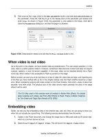
A theoretical head-and-shoulders top formation is described in Figure
3.1. The first clue of weakness in the is provided by prices reversing
at 1 from their previous highs to form a left shoulder. A second rally at 2
causes prices to surpass their earlier highs established at forming a head
at 3. Ideally, the volume on the second rally to the head should be lower
than the volume on the first rally to the left shoulder. A reaction from this
rally takes prices lower, to a level near 2, but in any event to a level below

the top of the left shoulder at 1. This is denoted by 4.
A third rally ensues, on decidedly lower volume than that accom-
panying the preceding two rallies, which helped form the left shoulder
and the head. This rally fails to reach the height of the head before yet
another pullback occurs, setting off a right shoulder formation. If the
third rally takes prices above the head at 3, we have what is known as
a broadening top formation rather than a head-and-shoulders reversal.
Therefore, a chartist ought not to assume that a head-and-shoulders for-
mation is in place simply because he observes what appears to be a left
shoulder and a head. This is particularly important, since broadening
top formations do not typically obey the same measuring objectives as
do head-and-shoulders reversals.
Minimum Measuring Objective
the third rally fizzles out before reaching the head, and if prices
on the third pullback close below an imaginary line connecting points
26
ESTIMATING RISK AND REWARD
Head
Minimum
measuring
objective
Figure
3.1
Theoretical head-and-shoulders pattern.
2 and 4, known as the “neckline,” on heavy volume and increasing open
interest, a head-and-shoulders top is in place. If prices close below the
neckline, they can be expected to fall from the point of penetration by a
distance equal to that from the head to the neckline. This is a minimum
measuring objective.
While it is possible that prices might continue to head downward, it is

equally likely that a pullback might occur once the minimum measuring
HEAD-AND-SHOULDERS FORMATION 27
objective has been met. Accordingly, at this point the trader might
want to lighten the position if he or she is trading multiple con-
tracts.
Estimated Risk
The trend line connecting the head and the right shoulder is called a
“fail-safe line.” Depending on the shape of the formation, either the
neckline or the fail-safe line could be farther from the entry point. A
protective stop-loss order should be placed just beyond the farther of
the two trendlines, allowing for a minor retracement of prices without
getting needlessly stopped out.
Two Examples of Head-and-Shoulders Formations
Figure gives an example of a head-and-shoulders bottom formation
in July 1991 silver. Here we, have a downward-sloping neckline, with
the distance from the head to the neckline approximately equal to 60
cents. Measured from a breakout at 418 cents, this gives a minimum
measuring objective of 478 cents. The fail-safe line (termed fail-safe
line 1 in Figure connecting the bottom of the head and the right
shoulder (right shoulder 1) recommends a sell-stop at 399 cents. At the
breakout of 418 cents, we have the possibility of earning 60 cents while
assuming a risk. This yields a reward/risk ratio of 3.16. The
breakout does occur on April 18, but the trader is promptly stopped out
the same day on a slump to 398 cents.
After the sharp plunge on April 18, prices stabilize around 390 cents,
forming yet another right shoulder (right shoulder 2) between April 19
and May 6. Extending the earlier neckline, we have a new breakout point
of 412 cents. The new fail-safe line (termed fail-safe line 2 in Figure
recommends setting a sell-stop of 397 cents. At the breakout of 412
cents, we now have the possibility of earning 60 cents while assuming a

risk, for a reward/risk ratio of 4.00. In subsequent action, July
silver rallies to 464 cents on July 7, almost meeting the target of the
head-and-shoulders bottom.
In Figure we have an example, in the September 1991 S&P
Index futures, of a possible head-and-shoulders top formation that
did not unfold as expected. The head was formed on April 17 at 396.20,
500
450
400
350
300
10000
90
Jan 91 Feb
Mar
Jun
Jul
Figure
Head-and-shoulders formations: (a) bottom in July 1991 silver.
90
Jan 91 Feb
Mar
Jun
Jul
100
375
350
325
300
10000

Figure
Head-and-shoulders formations: possible top in September 1991 S&P 500
Index.
30
ESTIMATING RISK AND REWARD
with a possible left shoulder formed at 387.75 on April 4 and the right
shoulder formed on May 9 at 387.80. The head-and-shoulders top was
set off on May 14 on a close below the neckline. However, prices broke
through the fail-safe line connecting the head and the right shoulder on
May 28, stopping out the short trade and negating the hypothesis of a
head-and-shoulders top.
DOUBLE TOPS AND BOTTOMS
A double top is formed by a pair of peaks at approximately the same
price level. Further, prices must close below the low established between
the two tops before a double top formation is activated. The retreat
from the first peak to the valley is marked by light volume. Volume
picks up on the ascent to the second peak but falls short of the volume
accompanying the earlier ascent. Finally, we see a pickup in volume as
prices decline for a second time. A double bottom is simply a double top
turned upside down, with the foregoing rules, appropriately modified,
equally applicable.
As a rule, a double top formation is an indication of bearishness, es-
pecially if the right half of the double top is lower than the left half. Sim-
ilarly, a double bottom formation is bullish, particularly if the right half
of the double bottom is higher than the left half. The market unsuccess-
fully attempted to test the previous peak (trough), signalling bearishness
(bullishness).
Minimum Measuring Objective
In the case of a double top, it is reasonable to expect that the decline
will continue at least as far below the imaginary support line connecting

the two tops as the distance from the higher of the twin peaks to the
support line. Therefore, the greater the distance from peak to valley,
the greater the potential for the impending reversal. Similarly, in the
case of a double bottom, it is safe to assume that the upswing will
continue at least as far up from the imaginary resistance line connecting
the two bottoms as the height from the lower of the double bottoms
to the resistance line. Once this minimum objective has been met, the
trader might want to set a tight protective stop to lock in a significant
portion of the unrealized profits.
DOUBLE TOPS AND BOTTOMS
Estimated Risk
31
The imaginary line drawn as a tangent to the valley connecting two tops
serves as a reliable support level. Similarly, the tangent to the peak con-
necting two bottoms serves as a reliable resistance level. Accordingly, a
trader might want to set a stop-loss order just above the support level,
in case of a double top, or just below the resistance level, in case of
a double bottom. The goal is to avoid falling victim to minor
ments, while at the same time guarding against unanticipated shifts in
the underlying trend.
If the closing price of the day that sets off the double top or bottom
formation substantially overshoots the hypothetical support or resistance
level, the potential reward on the trade might barely exceed the estimated
risk. In such a situation, a trader might want to wait for a pullback before
initiating the trade, in order to attain a better reward/risk ratio.
Two Examples of a Double Top Formation
Consider the December 1990 soybean oil chart in Figure 3.3. We have
a top at 25.46 cents formed on July 2, with yet another top formed
on August 23 at 25.55. The valley high on July 23 was 23.39 cents,
representing a distance of 2.16 cents from the peak of 25.55 on August

23. This distance of 2.16 cents measured from the valley high of 23.39
cents, represents the minimum measuring objective of 21.23 cents for
the double top. The double top is set off on a close below 23.39 cents.
This is accomplished on October 1 at 22.99. The buy stop for the trade
is set at 23.51, just above the high on that day, for a risk of 0.52 cents.
The difference between the entry price, 22.99 cents, and the target
price, 21.23 cents, gives a reward estimate of 1.76 cents for an associ-
ated risk of 0.52 cents. A reward/risk ratio of 3.38 suggests that this is
a highly desirable trade. After the minimum reward target was met on
November 6, prices continued to drift lower to 19.78 cents on November
20, giving the trader a bonus of 1.45 cents.
Although the comments for each pattern discussed here are illustrated
with the help of daily price charts, they are equally applicable to weekly
charts. Consider, for example, the weekly Standard Poor’s 500 (S&P
500) Index futures presented in Figure 3.4. We observe a double top
formation between August 10 and October 5, 1987, labeled A and B
in the figure. Notice that the left half of the double top, A, is higher than
19.5”
10000
0 24 7
21
May 90
Jun
Jul
Nov
Jan 91
Figure 3.3
Double top formation in December 1990 soybean oil.
AMJJASONDJFMAMJJASONDJFMAMJJASONDJFMAMJJ
87

88 89 90
375
325
275
225
Figure 3.4 Double top and triple bottom formation in weekly S&P 500 Index futures.
34
ESTIMATING RISK AND REWARD
the right half, B. The failure to test the high of 339.45, achieved by
A on August 24, 1987, is the first clue that the market has lost upside
momentum. A bearish close for the week of October 5, just below the
valley connecting the twin peaks,
confirms the double top formation.
The minimum measuring objective is given by the distance from peak
A to valley, approximately 20 index points. Measured from the entry
price of 312.20 on October 5, we have a reward target of 292.20. This
objective was surpassed during the week of October 12, when the index
closed at 282.25. Accordingly, the buy stop could be lowered to 292.20,
locking in the minimum anticipated reward. The meltdown that ensued
on October 19, Black Monday, was a major, albeit unexpected, bonus!
Triple Tops
and Bottoms
A triple top or bottom works along the same lines as a double top or
bottom, the only difference being that we have three tops or bottoms
instead of two. The three highs or lows need not be equally spaced, nor
are there any specific guidelines as regards the time that ought to elapse
between them. Volume is typically lower on the second rally or dip and
even lower on the third. Triple tops are particularly powerful as indicators
of impending bearishness if each successive top is lower than the preced-
ing top. Similarly, triple bottoms are powerful indicators of impending

bullishness if each successive bottom is higher than the preceding one.
In Figure 3.4, we see a classic triple bottom formation developing in
the weekly S&P 500 Index futures between May and November 1988,
marked C, D, and E. Notice how E is higher than D, and D higher than C,
suggesting strength in the stock market. This is substantiated by the speed
with which the market rallied from 280 to 360 index points, once the triple
bottom was established at E and resistance was surmounted at 280.
SAUCERS AND ROUNDED TOPS AND BOTTOMS
A saucer top or bottom is formed when prices seem to be stuck in a
very narrow trading range over an extended period of time. Volume
should gradually ebb to an extreme low at the peak of a saucer top or
at the trough of a saucer bottom if the pattern is to be trusted. As the
market seems to lack direction, a prudent trader would do well to stand
V-FORMATIONS, SPIKES, AND ISLAND REVERSALS
35
aside. As soon as a breakout occurs, the trader might want to enter a
position. Saucers are not too commonly observed. Moreover, they are
difficult to trade, because they develop at an agonizingly slow pace over
an extended period of time.
Minimum Measuring Objective and Permissible Risk
There are no precise measuring objectives for saucer tops and bottoms.
However, clues may be found in the size of the previous trend and in the
magnitude of retracement from previous support and resistance levels.
The length of time over which the saucer develops is also important.
Typically, the longer it takes to complete the rounding process, the more
significant the subsequent move is likely to be. The risk for the trade
is evaluated by measuring the distance between the entry price and the
stop-loss price, set just below (above) the saucer bottom (top).
An Example of a Saucer Bottom
Consider the October 1991 sugar futures chart in Figure 3.5. We have a

saucer bottom developing between the beginning of April and the first
week of June 1991, as prices hover around 7.50 cents. The breakout
past 8.00 cents finally occurs in mid-June, at which time a long position
could be established with a sell stop just below the life of contract lows
at 7.45 cents. After two months of lethargic action, a rally finally ignited
in early July, with prices testing 9.50 cents.
V-FORMATIONS, SPIKES, AND ISLAND REVERSALS
As the name suggests, a V-formation represents a quick turnaround
in the trend from bearish to bullish, just as an inverted V-formation
signals a sharp reversal in the trend from bullish to bearish. As Figure
3.6 illustrates, a V-formation could be sharply defined a spike, as in
Figure or as an island reversal, as in Figure Alternatively,
the formation may not be so sharply defined, taking time to develop
over a number of trading sessions, as in Figure
The chief prerequisite for a V-formation is that the trend preceding
it is very steep with few corrections along the way. The turn is charac-
terized by a reversal day, a key reversal day, or an island reversal day
on very heavy volume, as the V-formation causes prices to break through
V-FORMATIONS, SPIKES, AND ISLAND REVERSALS
37
Figure 3.6
Theoretical V-formations and island reversals: (a) spike
formation; (b) island reversal; (c) gradual V-formation.
a steep trendline. A reversal day downward is defined as a day when
prices reach new highs, only to settle lower than the previous day. Sim-
ilarly, a reversal day upward is one where prices touch new lows, only
to settle higher than the previous day. A key reversal day is one where
prices establish new life-of-contract highs (lows), only to settle lower
(or higher) than the previous day.
An island reversal, as is evident from Figure is so called because

it is flanked by two gaps: an exhaustion gap to its left and a breakaway
gap to its right. A gap occurs when there is no overlap in prices from
one trading session to the next.
Minimum Measuring Objective
The measuring objective for V-formations may be defined by reference
to the previous trend. At a minimum, a V-formation should retrace
anywhere between 38 percent and 62 percent of the move preceding
the formation, with 50 percent commonly used as a minimum reward
target. Once the minimum target is accomplished, it is quite likely
that a congestion pattern will develop as traders begin to realize their
38
ESTIMATING RISK AND REWARD
Estimated Risk
In the case of a spike or a gradual V-formation, a reasonable place to
set a protective stop would be just below the V-formation, for the start
of an or just above the inverted V-formation, for the start of a
downtrend. The logic is that once a peak or trough defined by a V-formation
is violated, the pattern no longer serves as a valid reversal signal.
In the case of an island reversal, a reasonable place to set a stop would
be just above the low of the island day, in the case of an anticipated
downtrend, or just below the high of the island day, in the case of an
anticipated The rationale is that once prices close the breakaway
gap that created the island formation, the pattern is no longer a legitimate
island and the trader must look for reversal clues afresh.
Examples of V-formations, Spikes, and Island Reversals
Figure 3.7 gives an example of V-formations in the March 1990 Trea-
sury bond futures contract. A reasonable buy stop would be at 101
for a sell signal triggered by the inverted V-formation in July 1989,
labeled A. Similarly, a reasonable sell stop would be just below 95
for the buy signal generated by the gradual V-formation, labeled B.

In both cases, the reversal signals given by the V-formations are ac-
curate.
However, if we continue further with the March 1990 Treasury bond
chart, we come across another case of a bearish spike at C. A trader
who decided to short Treasury bonds at 99-28 on December 15 with
a protective buy stop at 100-07 would be stopped out the next day as
the market touched 100-10. So much for the infallibility of spike days
as reversal patterns! We have yet another bearish spike developing on
December 20, denoted by D in the figure. Our trader might want to take
yet another stab at shorting Treasury bonds at 100-05 with a buy stop at
100-21. The risk is 16 ticks or $500 a contract-a risk well assumed,
as future events would demonstrate.
In Figure 3.8, we have two examples of an island reversal in July
1990 platinum futures. In November 1989, we have an island top. A
short position could be initiated on November 27 at $547.1, with a
protective stop just above $550.0, the low of the island top. This is
denoted by point A in the figure. In January 1990, we have an island
bottom, denoted by point B. A trader might want to buy platinum futures
SYMMETRICAL AND RIGHT-ANGLE TRIANGLES 41
the following day at $499.9, with a stop just below $489.0, the high of
the island reversal day. Notice that the island bottom is formed over a
two-day period, disproving the notion that islands must necessarily be
formed over a single trading session.
b.
SYMMETRICAL AND RIGHT-ANGLE TRIANGLES
A symmetrical triangle is formed by a series of price reversals, each
of which is smaller than its predecessor. For a legitimate symmetri-
cal triangle formation, we need to observe four reversals of the mi-
nor trend: two at the top and two at the bottom. Each minor top is
lower than the top formed by the preceding rally, and each minor bot-

tom is higher than the preceding bottom. Consequently, we have a
downward-sloping trendline connecting the minor tops and an
sloping trendline connecting the minor bottoms. The two lines inter-
sect at the apex of the triangle. Owing to its shape, this pattern is
also referred to as a “coil.” Decreasing volume characterizes the forma-
tion of a triangle, as if to affirm that the market is not clear about its
future course.
Normally, a triangle represents a continuation pattern. In exceptional
circumstances, it could represent a reversal pattern. While a continuation
breakout in the direction of the existing trend is most likely, a reversal
against the trend is possible. Consequently, avoid outguessing the mar-
ket by initiating a trade in the direction of the trend until price action
confirms a continuation of the trend by penetrating through the boundary
line encompassing the triangle. Ideally, such a penetration should occur
on heavy volume.
A right-angle triangle is formed when one of the boundary lines con-
necting the two minor peaks or valleys is flat or almost horizontal, while
the other line slants towards it. If the top of the triangle is horizontal
and the bottom converges upward to form an apex with the horizontal
top, we have an ascending right-angle triangle, suggesting bullishness in
the market. If the bottom is horizontal and the top of the triangle slants
down to meet it at the apex, the triangle is a descending right-angle
triangle, suggesting bearishness in the market.
Right-angle triangles are similar to symmetrical triangles but are sim-
pler to trade, in that they do not keep the trader guessing about their
intentions as do symmetrical triangles. Prices can be expected to ascend
42
ESTIMATING RISK AND REWARD
out of an ascending right-angle triangle, just as they can be expected to
descend out of a descending right-angle triangle.

Minimum Measuring Objective
The distance prices may be expected to move once a breakout occurs
from a triangle is a function of the size of the triangle pattern. For a
symmetrical triangle, the maximum vertical distance between the two
converging boundary lines represents the distance prices should move
once they break out of the triangle.
The farther out prices drift into the apex of the triangle without burst-
ing through the boundaries, the less powerful the triangle formation. The
minimum measuring objective just stated will ensue with the highest
probability if prices break out decisively at a point before three-quarters
of the horizontal distance from the left-hand corner of the triangle to the
apex.
The same measuring rule is applicable in the case of a right-angle
triangle. However, an alternative method of arriving at measuring ob-
jectives is possible, and perhaps more convenient, in the case of
angle triangles. Assuming we have an ascending right-angle triangle,
draw a line sloping upward parallel to the bottom boundary from the top
of the first rally that initiated the pattern. This line slopes upward to the
right, forming an upward-sloping parallelogram. At a minimum, prices
may be expected to climb until they reach the uppermost corner of the
parallelogram.
In the case of a descending right-angle triangle, draw a line par-
allel to the top boundary from the bottom of the first dip. This line
slopes downward to the right, forming a downward-sloping parallelo-
gram. Prices may be expected to drop until they reach the lowermost
corner of the parallelogram.
Estimated Risk
A logical place to set a protective stop-loss order would be just above the
apex of the triangle for a breakout on the downside. Conversely, for a
breakout on the upside, a protective stop-loss order may be set just below

the apex of the triangle. The dollar value of the difference between the
entry price and the stop price represents the permissible risk per con-
tract.
WEDGES
43
Example of a Triangle Formation
In Figure 3.8, we have an example of a symmetrical and a right-angle
triangle formation in the July 1990 platinum futures, marked C and
respectively. In both cases, the breakout is to the downside, and in
both cases the minimum measuring objective is attained and surpassed.
permissible risk per contract.
WEDGES
A wedge is yet another continuation pattern in which price fluctuations
are confined within a pair of converging lines. What distinguishes a
wedge from a triangle is that both boundary lines of a wedge slope up
or down together, without being strictly parallel. In the case of a triangle,
it may be recalled that if one boundary line were upward-sloping, the
other would necessarily be flat or downward-sloping.
In the case of a rising wedge, both boundary lines slope upward
from left to right, but for the two lines to converge the lower line must
necessarily be steeper than the upper line. In the case of a falling wedge,
the two boundary lines slant downward from left to right, but the upper
boundary line is steeper than the lower line.
A wedge normally takes between two and four weeks to form, during
which time volume is gradually diminishing. Typically, a rising wedge is
a bearish sign, particularly if it develops in a falling market. Conversely,
a falling wedge is bullish, particularly if it develops in a rising mar-
ket.
Minimum Measuring Objective
Once prices break out of a wedge, the expectation is that, at a minimum,

they will retrace the distance to the point that initiated the wedge. In
a falling wedge, the up move may be expected to take prices back
to at least the uppermost point in the wedge. Similarly, in a rising
wedge, the down move may be expected to take out the low point that
first started the wedge formation. Care must be taken to ensure that a
breakout from a wedge occurs on heavy volume. This is particularly
important in the case of a price breakout on the upside out of a falling
wedge.