Estimation of cosmic ray induced background and a fpga based data compression algorithm for deeme experiment
Bạn đang xem bản rút gọn của tài liệu. Xem và tải ngay bản đầy đủ của tài liệu tại đây (4.1 MB, 118 trang )
Estimation of Cosmic Ray Induced Background and
a FPGA-Based Data Compression Algorithm for
DeeMe Experiment
Nguyen Minh Truong
Department of Physics
Osaka University
This dissertation is submitted for the degree of
Doctor of Science
Graduate School of Science
May 2017
I would like to dedicate this thesis to my loving parents. Without their love, support and
putting me through the best education possible, I wouldn’t have been able to get to this stage.
To my wife, for her unending support and love, I wouldn’t have gotten through this doctorate
if it wasn’t for her.
Declaration
I hereby declare that the contents of this thesis are original except where specific reference
is made to the work of others, and they have not been submitted in whole or in part for any
other degree or any other university. This thesis is my own work and contains nothing which
is the outcome of work done in collaboration with others, except as specified in the text and
Acknowledgements.
Nguyen Minh Truong
May 2017
Acknowledgements
First of all, I would like to thank my advisors Prof. Masaharu Aoki and Prof. Yoshitaka Kuno
for the continuous support of my doctoral study and related research. Without Prof. Kuno’s
help, I can not study in Osaka University. Studying in Kuno-lab 7 years, from master course
until now, I really thank his favors. I also learn a lot from him. By giving clear answers for
my questions, he helps me open my mind in the best ways. Prof. Aoki is my main supervisor
in doctoral course, I learn from him a lot of knowledge, from the basic knowledge in physics,
computer and electronics areas. I realy admire him for his patience. I can not imagine how
much time he spend to teach me many things, from basic one to the depth knowledge.
Besides my advisors, I would like to thank the rest of my thesis committee: Prof.
Masaharu Nomachi, Prof. Tadafumi Kishimoto, and Prof. Takashi Nakano. By giving the
insightful comments and encouragement, and also the hard questions, they help me widen
my research from various perspectives. So, I can complete my thesis in the best ways.
My sincere thanks also goes to Prof. Youichi Igarashi, Prof. Yoshihiro Seiya, Dr. Hiroaki
Natori, Dr. Yohei Nakatsugawa and DeeMe collaborator, who provided me an opportunity to
join DeeMe group. Without their precious support, I can not finish my research.
I thank my fellow labmates, for friendship and for all the fun we have had in the last
five years. I realy thank my friends in Kuno-lab, with their help in Japanese whenever I have
problem with Japanese communication. I also thank my friends from Osaka City Univeristy,
for their helps in DeeMe beam time, for their comments in meeting and for all thing we have
in DeeMe group.
I am also thankfull to Kuno-lab secretaries, Ms. Miki, Ms. Komai, and Ms. Imoto. They
help me a lot during I study in Osaka Univeristy.
I would like to thank the Matsuda Yosahichi Memorial scholarship, for their financial
support for my study time in Japan.
Last but not the least, I would like to thank my family: my parents and my brother for
supporting me spiritually throughout writing this thesis and my life.
And huge thanks, love to my wife, a sky of my life.
Abstract
DeeMe experiment which is an experiment searching for muon to electron conversion
(µ-e conversion) will be conducted at J-PARC Materials and Life Science Experimental
Facility (MLF). The µ-e conversion in the nuclear field, µ − +N→ e− + N, is one of chargedLepton Flavor Violation (cLFV) processes. This process is forbidden in the Standard Model
(SM) of particle physics. However in the prediction of numerous theoretical models beyond
the SM, this process will happen at a level of few orders of magnitude below upper limits
given by previous experiments. The current upper limits of the branching ratio on the
µ-e conversion process are BR(µ − +Au→ e− +Au) < 7 × 10⁻¹³ given by SINDRUM II
experiment; BR(à +Ti e +Ti) < 4.3 ì 1012 and 4.6 × 10⁻¹² given by SINDRUM II
and the experiment at TRIUMF, respectively.
DeeMe experiment will use the pulsed proton beam from Rapid Cycling Synchrotron at
J-PARC. Electrons from µ-e conversion may be produced inside a production target and they
will be transported to a spectrometer by a secondary beamline. The momenta of electrons
will be measured by the spectrometer. DeeMe experiment has a potential to reach a single
event sensitivity (SES) at a level of 10−15 . The physics run will start to take data in around
2016−2017 when the construction of beamline at MLF has completed.
In order to achieve the SES written above, it is very important to understand and control
potential backgrounds. Cosmic ray induced background is one of potentially backgrounds
in DeeMe experiment. A Monte-Carlo study has performed to estimate its rate. Based on
this result, a data acquisition (DAQ) system has been developed so that it is not only used to
collect the detector signals from the spectromenter but also used to monitor the cosmic ray
induced background.
In this thesis, the Monte-Carlo study to estimate the cosmic ray induced background
and the DAQ system that can collect the detecotor signals and monitor the backgrounds are
reported.
Table of contents
List of figures
xv
List of tables
xix
1
2
3
Introduction
1.1 Overview . . . . . . . . . . . . .
1.2 Muon and Lepton Numbers . . . .
1.3 µ-e Conversion Process . . . . . .
1.4 How to Search for µ-e Conversion
1.5 µ-e Conversion Experiment . . . .
DeeMe experiment at J-PARC
2.1 Pulsed Proton Beam . . . . . . . .
2.2 Muon Production Target . . . . .
2.3 H-line at MLF . . . . . . . . . . .
2.4 Multi-Wire Proportional Chamber
2.5 Single Event Sensitivity . . . . . .
.
.
.
.
.
.
.
.
.
.
.
.
.
.
.
.
.
.
.
.
.
.
.
.
.
.
.
.
.
.
.
.
.
.
.
.
.
.
.
.
.
.
.
.
.
.
.
.
.
.
.
.
.
.
.
.
.
.
.
.
.
.
.
.
.
.
.
.
.
.
.
.
.
.
.
.
.
.
.
.
.
.
.
.
.
.
.
.
.
.
.
.
.
.
.
.
.
.
.
.
.
.
.
.
.
.
.
.
.
.
.
.
.
.
.
.
.
.
.
.
.
.
.
.
.
.
.
.
.
.
.
.
.
.
.
.
.
.
.
.
.
.
.
.
.
.
.
.
.
.
.
.
.
.
.
.
.
.
.
.
Background Estimation by Monte-Carlo Calculation
3.1 Overview . . . . . . . . . . . . . . . . . . . . . . . . . . . . .
3.2 Cosmic Ray Induced Background . . . . . . . . . . . . . . . .
3.2.1 Cosmic Ray Source . . . . . . . . . . . . . . . . . . . .
3.2.2 Cosmic Ray Induced Background in DeeMe Experiment
3.3 Monte Carlo Estimation . . . . . . . . . . . . . . . . . . . . . .
3.3.1 Coordinates Definition . . . . . . . . . . . . . . . . . .
3.3.2 Major Background Source Positions along H-line . . . .
3.3.3 Muon Interaction and Electron Production Mechanism .
3.3.4 Electron Production Models . . . . . . . . . . . . . . .
3.3.5 Electrons Induced at Horizontal Direction . . . . . . . .
.
.
.
.
.
.
.
.
.
.
.
.
.
.
.
.
.
.
.
.
.
.
.
.
.
.
.
.
.
.
.
.
.
.
.
.
.
.
.
.
.
.
.
.
.
.
.
.
.
.
.
.
.
.
.
.
.
.
.
.
.
.
.
.
.
.
.
.
.
.
.
.
.
.
.
.
.
.
.
.
.
.
.
.
.
.
.
.
.
.
.
.
.
.
.
.
.
.
.
.
.
.
.
.
.
1
1
2
3
5
7
.
.
.
.
.
11
12
12
15
18
20
.
.
.
.
.
.
.
.
.
.
23
23
26
26
27
28
29
30
37
40
42
xii
Table of contents
3.4
4
3.3.6 Event Generation . . . . . . . . . . .
3.3.7 Analysis and Event Cut . . . . . . . .
3.3.8 Cosmic Ray Induced Background . .
3.3.9 Systematic Errors . . . . . . . . . . .
Monitoring the Backgrounds . . . . . . . . .
3.4.1 Concept . . . . . . . . . . . . . . . .
3.4.2 Significance with Likelihood method
.
.
.
.
.
.
.
.
.
.
.
.
.
.
.
.
.
.
.
.
.
.
.
.
.
.
.
.
.
.
.
.
.
.
.
.
.
.
.
.
.
.
.
.
.
.
.
.
.
.
.
.
.
.
.
.
.
.
.
.
.
.
.
.
.
.
.
.
.
.
.
.
.
.
.
.
.
.
.
.
.
.
.
.
.
.
.
.
.
.
.
FPGA-Based Data Compressor
4.1 Overview . . . . . . . . . . . . . . . . . . . . . . . . . . . . . . . .
4.2 FADC board . . . . . . . . . . . . . . . . . . . . . . . . . . . . . . .
4.2.1 Hardware of the FADC Board . . . . . . . . . . . . . . . . .
4.2.2 Issue of the FADC Board . . . . . . . . . . . . . . . . . . .
4.3 Data Compression . . . . . . . . . . . . . . . . . . . . . . . . . . . .
4.3.1 Lossy Data Compression . . . . . . . . . . . . . . . . . . . .
4.3.2 Lossless Data Compression . . . . . . . . . . . . . . . . . .
4.4 Optimum Compression Method for DeeMe Experiment . . . . . . . .
4.5 Adaptive Delta Compression . . . . . . . . . . . . . . . . . . . . . .
4.5.1 Adaptive Delta Compression Algorithm . . . . . . . . . . . .
4.5.2 Data Format for Adaptive Delta Compression in FADC Board
4.5.3 Design of the Delta Compressor Module . . . . . . . . . . . .
4.5.4 Advantage of Delta Compressor Module . . . . . . . . . . .
4.6 Implementation to the FADC Board . . . . . . . . . . . . . . . . . .
4.6.1 Design of the Firmware . . . . . . . . . . . . . . . . . . . .
4.6.2 Data Format . . . . . . . . . . . . . . . . . . . . . . . . . .
4.6.3 Handshake Protocol between Modules . . . . . . . . . . . . .
4.6.4 Advantage of the New Firmware . . . . . . . . . . . . . . . .
4.7 Self Trigger . . . . . . . . . . . . . . . . . . . . . . . . . . . . . . .
4.8 Single FADC Board Performance Test . . . . . . . . . . . . . . . . .
4.8.1 Test the Compressor in FPGA . . . . . . . . . . . . . . . . .
4.8.2 Test Handshake Protocol . . . . . . . . . . . . . . . . . . . .
4.8.3 Test the Connection Between FADC Chip and FPGA Chip . .
4.8.4 Test Performance of New Firmware and Compressor . . . . .
4.9 Multiple-Board Performance Test . . . . . . . . . . . . . . . . . . .
4.9.1 Network Congestion . . . . . . . . . . . . . . . . . . . . . .
4.9.2 Head-of-Line Blocking Problem . . . . . . . . . . . . . . . .
4.9.3 High Performance Network Switch . . . . . . . . . . . . . .
.
.
.
.
.
.
.
.
.
.
.
.
.
.
.
.
.
.
.
.
.
.
.
.
.
.
.
.
.
.
.
.
.
.
.
.
.
.
.
.
.
.
.
.
.
.
.
.
.
.
.
.
.
.
.
.
.
.
.
.
.
.
.
.
.
.
.
.
.
.
.
.
.
.
.
.
.
46
47
51
52
53
53
54
.
.
.
.
.
.
.
.
.
.
.
.
.
.
.
.
.
.
.
.
.
.
.
.
.
.
.
.
57
57
58
58
59
61
61
62
68
70
70
74
76
80
81
81
84
87
88
89
91
91
93
94
96
97
97
98
99
Table of contents
xiii
5
103
Summary and Discussion
References
105
List of figures
1.1
1.2
1.3
1.4
1.5
µ-e conversion with photonic mechanism and non-photonics mechanism.
µ ± → e± γ and µ ± → e± e+ e− process with photonic mechanism. . . . .
The historical search of cLFV [18]. . . . . . . . . . . . . . . . . . . . . .
Setup of SINDRUM II experiment [20]. . . . . . . . . . . . . . . . . . .
SINDRUM II experiment result [20]. . . . . . . . . . . . . . . . . . . . .
.
.
.
.
.
4
5
8
8
9
2.1
2.2
2.3
The concept of DeeMe experiment. . . . . . . . . . . . . . . . . . . . . . .
Time structure of pulsed proton beam from RCS. . . . . . . . . . . . . . .
The ratio between the µ-e conversion branching ratio and the µ-e conversion
braching ratio on Al target is plotted as a function of atomic number Z [24].
Lifetime of negative muon in material is plotted as a function of atomic
number Z [16]. . . . . . . . . . . . . . . . . . . . . . . . . . . . . . . . .
The H-line and spectrometer in DeeMe experiment. . . . . . . . . . . . . .
The H-line beam envelope. . . . . . . . . . . . . . . . . . . . . . . . . . .
The acceptance of H-line [29]. . . . . . . . . . . . . . . . . . . . . . . . .
The concept of the MWPC. . . . . . . . . . . . . . . . . . . . . . . . . . .
Signal of MWPC in beam test at MLF November 2015. . . . . . . . . . . .
11
12
2.4
2.5
2.6
2.7
2.8
2.9
3.1
3.2
3.3
3.4
3.5
3.6
3.7
3.8
Momentum distribution of electrons produced by 3-GeV protons hitting a
Graphite target. . . . . . . . . . . . . . . . . . . . . . . . . . . . . . . . .
Time structure of charged particles at J-PARC MLF. . . . . . . . . . . . . .
Cosmic ray flux from various experiments [36]. . . . . . . . . . . . . . . .
Cosmic ray induced background in DeeMe experiment. . . . . . . . . . . .
Coordinate definition for cosmic ray induced background study. . . . . . .
Angles definition for cosmic ray induced background study. . . . . . . . . .
The concept of major background source position study. . . . . . . . . . .
Number of positron hitting virtual detector as a function of x position along
the beam line. . . . . . . . . . . . . . . . . . . . . . . . . . . . . . . . . .
13
13
16
17
17
19
20
24
24
26
28
29
30
31
31
xvi
List of figures
3.9
3.28
3.29
3.30
3.31
Phase space of electron and positron beam at target, a−b: phase space of
electron beam emitted from target, c−d: phase space of positron beam
emitted from MWPC4. . . . . . . . . . . . . . . . . . . . . . . . . . . . .
Phase space of electron and positron beam at HQ beam duct, a−b: phase
space of electron beam emitted from target, c−d: phase space of positron
beam emitted from MWPC4. . . . . . . . . . . . . . . . . . . . . . . . .
Positron distribution in HQ beam duct virtual detector. . . . . . . . . . . .
Positron distribution in production target. . . . . . . . . . . . . . . . . . .
Electron stopping power in iron [39]. . . . . . . . . . . . . . . . . . . . . .
Geometrical configuration of the G4beamline calculation to study the number
of electrons induced by muons in material. . . . . . . . . . . . . . . . . . .
Number of electrons induced versus the iron thickness. . . . . . . . . . . .
The θe− distribution of electron with momentum from 80 MeV/c to 120
MeV/c in different muon energies. . . . . . . . . . . . . . . . . . . . . . .
The electron production models. . . . . . . . . . . . . . . . . . . . . . . .
Concept to study models with cosmic rays muon. . . . . . . . . . . . . . .
Cosmic muon source in G4beamline. . . . . . . . . . . . . . . . . . . . . .
The θµ distribution of cosmic ray muon and muon 4 GeV. . . . . . . . . . .
The θe− distribution of electron induced from different muon theta hitting
the beam duct model. . . . . . . . . . . . . . . . . . . . . . . . . . . . . .
The θe− distribution of electron induced from different muon theta hitting
the target model. . . . . . . . . . . . . . . . . . . . . . . . . . . . . . . .
PDF of beam duct. . . . . . . . . . . . . . . . . . . . . . . . . . . . . . .
PDF of target. . . . . . . . . . . . . . . . . . . . . . . . . . . . . . . . . .
Example putting electron in H-line at HQ. . . . . . . . . . . . . . . . . . .
Concept of background rejection by track fitting. . . . . . . . . . . . . . .
Phase-space y’ versus y of electrons induced background from the HQ beam
duct (blue color) and electrons µ-e signal from the target (red color) at plan
X0 . . . . . . . . . . . . . . . . . . . . . . . . . . . . . . . . . . . . . . .
Momentum distribution of the electron background induced at HQ beam duct.
Momentum distribution of the electron background induced at the target. .
Muon lifetime and background level. . . . . . . . . . . . . . . . . . . . . .
Concept to monitor cosmic ray induced background. . . . . . . . . . . . .
4.1
4.2
4.3
A FADC board is used for recording signal waveforms from MWPC. . . .
FADC board diagram. . . . . . . . . . . . . . . . . . . . . . . . . . . . . .
Zero-suppression example. . . . . . . . . . . . . . . . . . . . . . . . . . .
3.10
3.11
3.12
3.13
3.14
3.15
3.16
3.17
3.18
3.19
3.20
3.21
3.22
3.23
3.24
3.25
3.26
3.27
33
34
35
36
38
38
39
39
41
42
43
43
44
44
46
47
47
49
50
51
51
52
54
58
59
62
xvii
List of figures
4.4
4.5
4.6
4.7
4.8
4.9
4.10
4.11
4.12
4.13
4.14
4.15
4.16
4.17
4.18
4.19
4.20
4.21
4.22
4.23
4.24
4.25
Huffman tree example. . . . . . . . . . . . . . . . . . . . . . . . . . .
Artificially constructed waveform from MWPC for DeeMe experiment.
Concept of Delta Compressor module. . . . . . . . . . . . . . . . . . .
Block diagram of Delta Module. . . . . . . . . . . . . . . . . . . . . .
Block diagram of Encoder Module. . . . . . . . . . . . . . . . . . . . .
Block diagram of Packer Module. . . . . . . . . . . . . . . . . . . . .
New firmware of FADC board. . . . . . . . . . . . . . . . . . . . . . .
Data format of new firmware of FADC board. . . . . . . . . . . . . . .
Handshake protocol between modules. . . . . . . . . . . . . . . . . . .
Concept of self trigger. . . . . . . . . . . . . . . . . . . . . . . . . . .
Self trigger concept. . . . . . . . . . . . . . . . . . . . . . . . . . . . .
Counter signal. . . . . . . . . . . . . . . . . . . . . . . . . . . . . . .
Histogram of number sample point of counter signal. . . . . . . . . . .
Histogram of delta value of counter signal. . . . . . . . . . . . . . . . .
Test fit input signal with the FADC board. . . . . . . . . . . . . . . . .
Spike problem of FADC board. . . . . . . . . . . . . . . . . . . . . . .
Test FADC board with DeeMe signal. . . . . . . . . . . . . . . . . . .
Test data transfer with two FADC boards. . . . . . . . . . . . . . . . .
Head of Line Blocking problem. . . . . . . . . . . . . . . . . . . . . .
Two VLAN set up for 12 FADC boards. . . . . . . . . . . . . . . . . .
Data transfer rate of 12 FADC boards. . . . . . . . . . . . . . . . . . .
DAQ screen with of 12 FADC boards. . . . . . . . . . . . . . . . . . .
.
.
.
.
.
.
.
.
.
.
.
.
.
.
.
.
.
.
.
.
.
.
. 64
. 69
. 76
. 77
. 78
. 79
. 82
. 86
. 88
. 89
. 90
. 92
. 92
. 93
. 94
. 95
. 97
. 98
. 99
. 100
. 101
. 101
List of tables
1.1
1.2
Properties of Leptons. . . . . . . . . . . . . . . . . . . . . . . . . . . . . .
Energy of µ-e conversion electrons. . . . . . . . . . . . . . . . . . . . . .
3
6
2.1
2.2
2.3
The strengths of production of muonic atom. . . . . . . . . . . . . . . . . .
The properties of C (graphite), Si and SiC. . . . . . . . . . . . . . . . . . .
Parameters of MWPC. . . . . . . . . . . . . . . . . . . . . . . . . . . . .
14
15
19
3.1
3.2
3.3
3.4
25
27
32
3.7
3.8
3.9
3.10
Major backgrounds in DeeMe experiment. . . . . . . . . . . . . . . . . . .
The factor fµ for muon angle from 70° to 87° . . . . . . . . . . . . . . . . .
Number of positron hitting the beam duct from inside. . . . . . . . . . . . .
Number of electrons induced with electrons momentum from 80 MeV/c to
120 MeV/c, 1.3 radian< θe− < 1.9 radian and -0.5 radian < φe− < 0.5 radian
in different cosmic ray muons angle. . . . . . . . . . . . . . . . . . . . . .
The expected number of cosmic ray muons come to areas and the electrons
induced from the cosmic ray muon hitting. . . . . . . . . . . . . . . . . . .
The number of electron passing through 4 MWPCs and the cosmic ray
induced background for DeeMe experiment. . . . . . . . . . . . . . . . . .
The number of positron induced by the cosmic ray. . . . . . . . . . . . . .
Background removed by applying the selection region. . . . . . . . . . . .
Background value and time analysis window. . . . . . . . . . . . . . . . .
Significance and monitor background time window. . . . . . . . . . . . . .
4.1
4.2
4.3
4.4
4.5
4.6
4.7
Spartan-6 XC6SLX150. . . . . . . . . . . . . .
Huffman table example. . . . . . . . . . . . . .
Huffman code example. . . . . . . . . . . . . .
LZW code example. . . . . . . . . . . . . . . .
Delta coding example. . . . . . . . . . . . . .
Compression ratios for the simulated waveform.
∆AVG and NBIT-DELTA. . . . . . . . . . . . .
59
63
65
67
68
69
72
3.5
3.6
.
.
.
.
.
.
.
.
.
.
.
.
.
.
.
.
.
.
.
.
.
.
.
.
.
.
.
.
.
.
.
.
.
.
.
.
.
.
.
.
.
.
.
.
.
.
.
.
.
.
.
.
.
.
.
.
.
.
.
.
.
.
.
.
.
.
.
.
.
.
.
.
.
.
.
.
.
.
.
.
.
.
.
.
.
.
.
.
.
.
.
.
.
.
.
.
.
.
.
.
.
.
.
.
.
45
46
48
48
50
52
55
xx
List of tables
4.8
4.9
4.10
4.11
Example of 3-bit delta code based on two’s complement. . . . . . . . .
Example compression code. . . . . . . . . . . . . . . . . . . . . . . .
Data format of delta compressor in FADC board. . . . . . . . . . . . .
Resource consumption of the Delta Compressor module implemented
Spartan-6. . . . . . . . . . . . . . . . . . . . . . . . . . . . . . . . . .
4.12 Input/Output Signal of Module. . . . . . . . . . . . . . . . . . . . . . .
4.13 Network speed versus global busy signal. . . . . . . . . . . . . . . . .
4.14 Clock phase and spike problem. . . . . . . . . . . . . . . . . . . . . .
. .
. .
. .
in
. .
. .
. .
. .
72
73
75
81
87
94
96
Chapter 1
Introduction
1.1
Overview
Direct Emission of Electron from Muon-Electron conversion experiment [1] − DeeMe
experiment − is an experiment searching for muon to electron conversion (µ-e conversion)
in nuclear field at single event sensitivity (SES) of 10−14 . It was proposed at the Japan Proton
Accelerator Research Complex (J-PARC) and will be performed at Materials and Life Science
Experimental Facility (MLF) H-line. The µ-e conversion process is one of charged-Lepton
Flavour Violation (cLFV) processes. The branching ratio of cLFV in the Standard Model
(SM) with the neutrino-oscillation extension is very small, at order of 10−52 [2, 3]. Therefore,
any experiments observing cLFV signal would provide us a clear evidence of new physics
beyond the SM and µ-e conversion experiment is considered as one of powerful probes to
search for cLFV.
The current upper limits on µ-e conversion is BR(µ − +Au→ e− +Au) < 7 ì 1013 [5]
by SINDRUM II; BR(à +Ti→ e− +Ti) < 4.3 × 10⁻¹² , 4.6 × 10⁻¹² [6] by SINDRUM II
and the experiment at TRIUMF, respectively. DeeMe experiment aims to search for µ-e
conversion signal in nuclear field better than the current upper limits. It was awarded Stage-2
approval from KEK/IMSS Program Advisory Commitee and it aims to start data taking in a
few years. With one year of physics data taking, it can achieve the Single Event Sensitivity
(SES) at 10−13 with a graphite production target. DeeMe experiment will use a proton beam
from Rapid Cycling Synchrotron (RCS), thus it will not interfere with any experiments which
use a main ring of J-PARC. It has a potential to reach the SES of 5 × 10⁻¹⁵ if the experiment
can run for 4 years with a SiC production target.
Cosmic ray induced background is one of potential backgrounds in DeeMe experiment.
Cosmic rays can pass through the ceiling of MLF, hit beam ducts or magnet yokes, and
produce electrons to horizontal direction. These electrons with momenta close to 105 MeV/c
2
Introduction
can be transported to a spectrometer and be mistaken for µ-e conversion signals. The
estimation of such a type of background is described in this thesis.
A data acquisition system suited for monitoring of cosmic-ray induced background has
been developed. The requirement to the monitoring system estimated with a Monte-Carlo
study and the data transfer performance are presented in this thesis.
This thesis is presented with a structure as follows: the physics motivation of DeeMe
experiment, normal muons decays in SM, cLFV and µ-e conversion are presented in the first
chapter. The second chapter is an overview of DeeMe experiment: idea, beamline, target,
tracker system and their requirements. Details of the cosmic ray induced background are
described in chapter 3. In chapter 4, details of the data acquisition system that enables us to
record both signals and potential backgrounds at the same time are described. The summary
and discussions are presented in chapter 5.
1.2
Muon and Lepton Numbers
Muons were discovered by Carl D. Andersion and Seth Neddermeyer [7] in 1936 when they
observed the cosmic-ray particle "showers." At the beginning, it was thought that muon was
a particle predicted by Yukawa Hideki in 1935 to explain the strong force in nuclei because
its mass, 200 times heavier than the mass of electron, was close to the one predicted by him.
However, this was not right, the particle which was predicted by Yukawa is a pion, and the
muon itself never contributes to strong interaction in nuclear field. The muon is a member of
a lepton group, unstable and quickly decays to an electron, a neutrino and an anti-neutrino
with a lifetime about 2.2 µs. As all elementary particles, the muon has an antiparticle with
the same mass and spin but the opposite charge; the muon has negative charge (-1e) and
the anti-muon has positive charge (+1e). The muon is also called the negative muon and is
denoted as µ − , the anti-muon is called the positive muon and is denoted as µ + .
Muon, electron, tau, and their associated neutrinos aggregate a group are called lepton
group. In the SM of particle physics, leptons, and quarks are elementary particles and
compose matter. Electron, muon, and tau are charged leptons and each of them has a negative
charge. Leptons respond with electromagnetic, weak, and gravitational forces but they do
not with strong interaction. They are fermions and each of them has a spin of 1/2.
In order to explain the absence of ν + n → p + e− , E. Konopinski and H. Mahmoud [4]
introduced lepton number. In addition, lepton family numbers − Le , Lµ , and Lτ − are also
introduced. Each leptons family numbers is equal to +1 for each lepton and -1 for each anti
lepton. Table 1.1 summarizes major properties of leptons. In the SM of particle physics, the
3
1.3 µ-e Conversion Process
Table 1.1 Properties of Leptons.
Name
Charge (e)
Lepton
number
e−
µ−
τ−
νe
νµ
ντ
-1
-1
-1
0
0
0
+1
+1
+1
+1
+1
+1
Lepton family
number
Le Là L
+1 0
0
0 +1
0
0
0
+1
+1 0
0
0 +1
0
0
0
+1
Mass (MeV/c2 )
Lifetime (ns)
0.511
105
1776
unknown
unknown
unknown
Stable
2197.019
2.906 ì104
unknown
unknown
unknown
lepton family number is conserved. For an example, in the decay of muon,
µ − → νµ + e− + νe ,
L
:1
=
1+1−1
Lµ
:1
=
1+0+0
Le
:0
=
0+1−1
the lepton number and lepton family numbers in the initial state should be equal to the final
state.
In contrast to this process, the conversion of muon to electron in nuclear field,
µ − + N → e− + N,
L
:1
+0 = 1
+0
Lµ
:1
+ 0 ̸= 0
+0
Le
:0
+ 0 ̸= 1
+0
apparently violates the lepton family numbers. Thus, in the SM of particle physics, this is
forbidden. It is noteworthy that the lepton number is conserved in this reaction.
1.3
µ-e Conversion Process
As mentioned in Section 1.2, the interaction that violates the lepton family numbers is
not allowed in the SM of particle physics and such interactions are called Lepton Flavor
4
Introduction
Violation (LFV) process. It should be noted that the neutrino with a certain lepton flavour at
birth changes its flavour while traveling in space: Lepton flavor is no longer conserved for
neutrinos. The LFV only happens for neutrino; the question is whether there is any LFV for
charged leptons (charged-Lepton Flavor Violation, cLFV). This question was raised in early
1940’s much before the establishment of neutrino flavors and physicists have been trying to
find any signals of cLFV.
After the discovery of the neutrino oscillation, the mass square differences of neutrinos
are confirmed to be non zero and the SM is extended with the neutrino oscillation. Based on
the extension of SM that includes the neutrino oscillation, the cLFV process is estimated to
be at the level of 10−52 [2, 3]. This level is too small for the present experimental technology.
This means the process of cLFV is still practically forbidden in the framework of the SM
with the extension of neutrino oscillation. Therefore, if any cLFV process is observed, it will
provide us a clear evidence for new physics beyond the SM.
Although cLFV is forbidden in the framework of the SM of particle physics, many
theoretical models beyond the SM predict that cLFV may happen at a level experimentally
accessible, a Left-Right seesaw model predicts 10−12 − 10−14 [10] and double charged
Higgs model predicts 10−13 − 10−14 [11], a Constrained Minimal Supersymmetric Standard
Model-seesaw predicts 10−14 − 10−18 [12].
There are many experimental methods to search for cLFV, such as µ ± → e± γ, µ-e
conversion, or µ ± → e± e+ e− and so on. In those experimental methods, µ-e conversion in
the nuclear field (µ − N → e− N) is considered as the most powerful probe to search for cLFV.
In theoretical point of view, there are two processes contributing to the reaction: photonic
and non-photonic mechanism. The photonic mechanism is mediated by exchanging photon
in an intermediate state. The non-photonic mechanism is mediated by various particles in
the intermediate state such as neutralino χ˜A0 , slepton l˜χ and squark q˜χ in the supersymmetry
(SUSY) model [21] or gauge boson X, W, etc in simplest little higgs (SLH) model [23]. The
µ-e conversion receives contributions from both non-photonic and photonic mechanisms,
so it is sensitive to a wide variety of models than the µ ± → e± γ that only sensitive to the
photonic mechanism.
e-
~
~-
χ
~0
A
γ
qj
~
l
µ
qj
(a) photonic mechanism [22].
q
e
~0
B
q~
q
(b) non-photonic mechanism [21].
Fig. 1.1 µ-e conversion with photonic mechanism and non-photonics mechanism.
5
1.4 How to Search for µ-e Conversion
e
µ
χ~-
γ
ℓ
~
ν
ℓi
(a) µ ± → e± γ process [22].
e
e
(b) µ ± → e± e+ e− process [21].
Fig. 1.2 µ ± → e± γ and µ ± → e± e+ e− process with photonic mechanism.
Figure 1.1 taken from [21], [22] shows example of Feynman diagram for µ-e conversion
with photonic mechanism and non-photonic mechanism at the quark level. The photonic
mechanism of µ-e conversion process is different from the µ ± → e± γ process that has a
photon emitting to the outside. It is also similar to the photonic process of µ ± → e± e+ e−
process, but they are different in the final production.
If the photonic mechanism is dominant, the branching ratio of µ-e conversion process is
smaller than one of µ ± → e± γ process by approximately a few hundred times. In contrast,
if the non-photonic mechanism is dominant, the branching ratio of µ ± → e± γ process is
smaller than one of µ-e conversion process. Therefore, the ratio of the branching ratios
between µ-e conversion process and µ ± → e± γ process provides important information that
influence on theories. Furthermore, because of the potential contribution of non-photonic
mechanism, the µ-e conversion process still has ability to be found at the branching ratio
where no signal of µ ± → e± γ has been found.
1.4
How to Search for µ-e Conversion
The search for µ-e conversion has been performed during later half of 19th century. In order
to measure electrons from µ-e conversion process, a muon beam is guided to a muon-stopping
target. The muon entered in the muon-stopping target is trapped in the atomic orbit of the
target nucleus and forms a muonic atom. After that, one of the following processes happens
in the framework of the SM of particle physics:
• muon decay in orbit (DIO): à e à e ,
ã muon capture: µ − + A(N, Z) → νµ + A(N, Z 1).
ã In addition to them, the à-e conversion process: µ − + A(N, Z) → e− + A(N, Z),
may happen if the cLFV exists.
Both the muon capture and the µ-e conversion process interact with nucleus in shortdistance thus the initial phase space factor is the same the overlap of the µ − and the nucleus.
6
Introduction
The µ-e conversion branching ratio (BR) is defined as the ratio to the muon capture
BR(µ − + A(N,Z) → e− + A(N,Z)) =
Γ(µ − + A(N,Z) → e− + A(N,Z))
,
Γ(µ − + A(N,Z) → νµ + A(N,Z-1)
(1.1)
where Γ is a partial decay width. Both DIO and µ-e conversion processes emit electrons but
the electron from µ-e conversion process has mono-energy
Eµe = mµ − Eb − Erecoil ,
(1.2)
where mµ is the muon mass; Eb is the binding energy of muonic atom which is ∼
E2
Z 2 α 2 mµ
;
2
and Erecoil is the energy of nuclear recoil which can approximate 2mµe ; and Z, α, mN are the
N
atomic number of nucleus, the fine-structure constant and the mass of nucleus, respectively.
Table 1.2 presents the values of Eµe for several materials. Carbon and silicon will be used as
a production target for DeeMe experiment.
In opposite, electrons emitted from DIO process have continuous energy distribution.
The maximum energy of standard muon decay µ − → e− νµ νe in free space is 52.8 MeV,
which is far below the µ-e conversion electron. However, in case of DIO, the maximum
energy of DIO electron is exactly the same to Eµe due to the existence of nuclear recoil
effect. This makes a little bit complicated to search for µ-e conversion signal. According
to O. Shanker [13], the energy spectrum of DIO electron near Eµe falls steeply with the
factor proportional to (Eµe − Ee )5 , where Ee is the energy of DIO electron. Thus, the
DIO background can be suppressed by improving the resolution of electron momentum
measurement.
Table 1.2 Energy of µ-e conversion electrons.
Material
C
Si
Al
Ti
Eµe (MeV)
105.1
105.0
105.0
104.2
The second thing that should be considered in µ-e conversion experiment is the timing
of the electron. To produce muon for µ-e conversion experiment, production target is bombarded with a proton beam. The bombardment also produces a large number of background
electrons around 105 MeV. For example, a proton produces π, π decays to µ and µ decays
to e in-flight with 105 MeV. The π 0 may also produce 105 MeV electrons through π 0 → γγ
7
1.5 µ-e Conversion Experiment
decay followed by γ conversion to e+ e− . They can be mis-identified as the electron from µ-e
conversion, and called prompt background. However, µ-e conversion process may happen
after muons are trapped by nuclei and formed muonic atoms, so µ-e conversion electrons
shall be emitted from muonic atoms with delayed timing from the initial muon. The lifetime
of muonic atoms is expressed as:
1
τtotallifetime
=
1
τdecay
+
1
τcapture
,
(1.3)
where τtotallifetime is the total lifetime of muonic atom, τdecay is the lifetime of free negative
muon decay and τcapture is the partial lifetime of muon capture process. In case of carbon
and silicon, their total lifetime are respectively 2.02 µs and 0.81 µs. Therefore, to remove
prompt backgrounds and detect µ-e conversion signal, it is needed to select delayed timing
to measure momentum of electron.
1.5
µ-e Conversion Experiment
As mentioned in Section 1.3, the µ-e conversion process is one of cLFV process and it
is considered as the most powerful tool to search for cLFV processes. From late 19th
century, the µ-e conversion signal has been searched with various experiments. It has
been performed together with µ ± → e± γ and µ ± → e± e+ e− experiments to look for cLFV
processes. However, these experiments did not find any signals of cLFV and upper limits
were set for these processes. Figure 1.3 taken from [18] shows the history of experiments
searching for cLFV with muon. From this figure, it it said that the upper limit of µ-e
conversion process has been updated during 50 years and the current upper limit is ∼ 10−13 .
The current upper limit of µ-e conversion was given by SINDRUM II experiment
at PSI [19]. Figure 1.4 taken from [20] shows a setup of SINDRUM II experiment. In
this experiment, 590 MeV proton beam with 1 MW from PSI ring cyclotron is used to
bombard the 40-mm carbon target and the πE5 beam line is used to transport secondary
particles (π, µ, e) to SINDRUM II spectrometer, which has an Au target, and the spectrometer
measured momenta of electrons emitted from the Au target.
After the analysis of data, SINDRUM II showed the result of momentum distribution of
electrons as shown in Figure 1.5. From this result, SINDRUM II group concluded that they
did not find any µ-e conversion signal and only observed a high energy component from pion
induced background [20]. Finally, the upper limit BR(à+Al e+Au) < 7 ì 1013 was set.
8
Introduction
Fig. 1.3 The historical search of cLFV [18].
Fig. 1.4 Setup of SINDRUM II experiment [20].
The result of SINDRUM II experiment was published in 2006. For 10 years, many
technologies have been developed and now the sensitivity of experiment can be increased
by applying these technologies. Three experiments are trying to search for µ-e conversion
signal now: Mu2e at USA, COMET at J-PARC and DeeMe experiment at J-PARC. On
these experiments, pulsed proton beams will be used to produce muons. It is different from
SINDRUM II experiment which used a continuous proton beam. They expect to remove
prompt backgrounds and have higher opportunity to find µ-e conversion signal.
1.5 µ-e Conversion Experiment
Fig. 1.5 SINDRUM II experiment result [20].
9
Chapter 2
DeeMe experiment at J-PARC
DeeMe experiment is an experiment to search for µ-e conversion at sensitivity of 10−14 ,
one or two orders of magnitude below the current upper limit [1]. This experiment will be
conducted at H-line of J-PARC Materials and Life Science Experimental Facility (MLF).
Figure 2.1 shows the concept of DeeMe experiment. The idea in DeeMe experiment is to use
muonic atoms produced in the proton target itself. Muonic atoms formed in the production
target may emit electrons through µ-e conversion process. These electrons are transferred to
a spectrometer by H-line while low energy background electrons will be removed during the
transportation. Momenta of electrons are measured by the spectrometer which consists of a
dipole magnet and four multi-wire proportional chambers (MWPCs).
Proton
Fig. 2.1 The concept of DeeMe experiment.
12
2.1
DeeMe experiment at J-PARC
Pulsed Proton Beam
In order to remove the prompt background for µ-e conversion search, DeeMe experiment will
use the pulsed proton beam. Three GeV pulsed proton beam from Rapid Cycling Synchrotron
(RCS) at J-PARC will be used to bombard the production target and produce muons. The
beam power of RCS is designed to be 1 MW and it will be injected to MLF with the repetition
rate of 25 Hz. It is also injected to a Main Ring in every 2.4 seconds.
3 GeV
Pulsed Proton
from RCS
600ns
600ns
time
200ns
40ms
Fig. 2.2 Time structure of pulsed proton beam from RCS.
Figure 2.2 shows the time structure of pulsed proton beam from RCS. It has a double
pulse structures with 200-ns width for each pulse and 600-ns separation between two pulses.
2.2
Muon Production Target
The material of the target should be optimized by taking into account the balance between
physics sensitivity, muonic atom yield, lifetime, etc. Figure 2.3 taken from [24] shows the Z
dependence of the ratio between the branching ratio µ-e conversion rate on different material
and the braching ratio µ-e rate on Al, R(Z) is calculated with Kitano method, the RWF (Z)
is calculated with Weinberg-Feinberg formula and the RS (Z) is calculated with Shanker’s
approximation. From these calculations, the branching ratio of µ-e conversion increases as
Z increase for the light nuclei such as Z < 30. It decreases as Z increases for heavy nuclei
Z > 60. Materials with Z= 30 ∼ 60 might be better than light Z to increase the physics
sensitivity for the photonic process.
Figure 2.4 shows the Z dependence of the lifetime of negative muon in material [16].
The lifetime of negative muon in the material decreases when the atomic number increases.
For the atomic number larger than 15, the lifetime of negative muon is smaller than 700 ns.
Considering the time structure of pulsed proton beam from RCS which has double pulse
structures with 600 ns separation, the best target material for DeeMe experiment should have
the atomic number smaller than 15 (Z < 15).
13
2.2 Muon Production Target
Fig. 2.3 The ratio between the µ-e conversion branching ratio
and the µ-e conversion braching ratio on Al target is plotted
as a function of atomic number Z [24].
2400
2200
2000
Lifetime (ns)
1800
1600
1400
1200
1000
800
600
400
200
0
0
20
40
Z
60
80
Fig. 2.4 Lifetime of negative muon in material
is plotted as a function of atomic number Z [16].
100