Tài liệu Microcontroller Based Applied Digital Control pdf
Bạn đang xem bản rút gọn của tài liệu. Xem và tải ngay bản đầy đủ của tài liệu tại đây (5.47 MB, 314 trang )
Microcontroller Based Applied Digital
Control
JWBK063-FM JWBK063-Ibrahim January 4, 2006 18:11 Char Count= 0
Microcontroller Based
Applied Digital Control
i
Microcontroller Based Applied Digital Control D. Ibrahim
C
2006 John Wiley & Sons, Ltd. ISBN: 0-470-86335-8
JWBK063-FM JWBK063-Ibrahim January 4, 2006 18:11 Char Count= 0
Microcontroller Based
Applied Digital Control
Dogan Ibrahim
Department of Computer Engineering
Near East University, Cyprus
iii
JWBK063-FM JWBK063-Ibrahim January 4, 2006 18:11 Char Count= 0
Copyright
C
2006 John Wiley & Sons Ltd, The Atrium, Southern Gate, Chichester,
West Sussex PO19 8SQ, England
Telephone (+44) 1243 779777
Email (for orders and customer service enquiries):
Visit our Home Page on www.wiley.com
All Rights Reserved. No part of this publication may be reproduced, stored in a retrieval system or transmitted in
any form or by any means, electronic, mechanical, photocopying, recording, scanning or otherwise, except under
the terms of the Copyright, Designs and Patents Act 1988 or under the terms of a licence issued by the Copyright
Licensing Agency Ltd, 90 Tottenham Court Road, London W1T 4LP, UK, without the permission in writing of the
Publisher. Requests to the Publisher should be addressed to the Permissions Department, John Wiley & Sons Ltd,
The Atrium, Southern Gate, Chichester, West Sussex PO19 8SQ, England, or emailed to , or
faxedto(+44) 1243 770620.
Designations used by companies to distinguish their products are often claimed as trademarks. All brand names and
product names used in this book are trade names, service marks, trademarks or registered trademarks of their
respective owners. The Publisher is not associated with any product or vendor mentioned in this book.
This publication is designed to provide accurate and authoritative information in regard to the subject matter
covered. It is sold on the understanding that the Publisher is not engaged in rendering professional services. If
professional advice or other expert assistance is required, the services of a competent professional should be sought.
Other Wiley Editorial Offices
John Wiley & Sons Inc., 111 River Street, Hoboken, NJ 07030, USA
Jossey-Bass, 989 Market Street, San Francisco, CA 94103-1741, USA
Wiley-VCH Verlag GmbH, Boschstr. 12, D-69469 Weinheim, Germany
John Wiley & Sons Australia Ltd, 42 McDougall Street, Milton, Queensland 4064, Australia
John Wiley & Sons (Asia) Pte Ltd, 2 Clementi Loop #02-01, Jin Xing Distripark, Singapore 129809
John Wiley & Sons Canada Ltd, 22 Worcester Road, Etobicoke, Ontario, Canada M9W 1L1
Wiley also publishes its books in a variety of electronic formats. Some content that appears
in print may not be available in electronic books.
Library of Congress Cataloging-in-Publication Data
Ibrahim, Dogan.
Microcontroller based applied digital control / Dogan Ibrahim.
p. cm.
ISBN 0-470-86335-8
1. Process control—Data processing. 2. Digital control systems—Design and construction. 3. Microprocessors.
I. Title.
TS156.8.I126 2006
629.8
9—dc22 2005030149
British Library Cataloguing in Publication Data
A catalogue record for this book is available from the British Library
ISBN-13 978-0-470-86335-0 (HB)
ISBN-10 0-470-86335-8 (HB)
Typeset in 10/12pt Times by TechBooks, New Delhi, India
Printed and bound in Great Britain by Antony Rowe Ltd, Chippenham, Wiltshire
This book is printed on acid-free paper responsibly manufactured from sustainable forestry
in which at least two trees are planted for each one used for paper production.
iv
JWBK063-FM JWBK063-Ibrahim January 4, 2006 18:11 Char Count= 0
Contents
Preface xi
1 Introduction 1
1.1 The Idea of System Control 1
1.2 Computer in the Loop 2
1.3 Centralized and Distributed Control Systems 5
1.4 Scada Systems 6
1.5 Hardware Requirements for Computer Control 7
1.5.1 General Purpose Computers 7
1.5.2 Microcontrollers 8
1.6 Software Requirements for Computer Control 9
1.6.1 Polling 11
1.6.2 Using External Interrupts for Timing 11
1.6.3 Using Timer Interrupts 12
1.6.4 Ballast Coding 12
1.6.5 Using an External Real-Time Clock 13
1.7 Sensors Used in Computer Control 14
1.7.1 Temperature Sensors 15
1.7.2 Position Sensors 17
1.7.3 Velocity and Acceleration Sensors 20
1.7.4 Force Sensors 21
1.7.5 Pressure Sensors 21
1.7.6 Liquid Sensors 22
1.7.7 Air Flow Sensors 23
1.8 Exercises 24
Further Reading 25
2 System Modelling 27
2.1 Mechanical Systems 27
2.1.1 Translational Mechanical Systems 28
2.1.2 Rotational Mechanical Systems 32
v
JWBK063-FM JWBK063-Ibrahim January 4, 2006 18:11 Char Count= 0
vi CONTENTS
2.2 Electrical Systems 37
2.3 Electromechanical Systems 42
2.4 Fluid Systems 44
2.4.1 Hydraulic Systems 44
2.5 Thermal Systems 49
2.6 Exercises 52
Further Reading 52
3 The PIC Microcontroller 57
3.1 The PIC Microcontroller Family 57
3.1.1 The 10FXXX Family 58
3.1.2 The 12CXXX/PIC12FXXX Family 59
3.1.3 The 16C5X Family 59
3.1.4 The 16CXXX Family 59
3.1.5 The 17CXXX Family 60
3.1.6 The PIC18CXXX Family 60
3.2 Minimum PIC Configuration 61
3.2.1 External Oscillator 63
3.2.2 Crystal Operation 63
3.2.3 Resonator Operation 63
3.2.4 RC Operation 65
3.2.5 Internal Clock 65
3.3 Some Popular PIC Microcontrollers 66
3.3.1 PIC16F84 Microcontroller 67
3.3.2 PIC16F877 Microcontroller 71
3.4 Exercises 75
Further Reading 76
4Programming PIC Microcontrollers in C 77
4.1 PICC Lite Variable Types 78
4.1.1 Bit 78
4.1.2 Unsigned Char 78
4.1.3 Signed Char 79
4.1.4 Unsigned Int 79
4.1.5 Signed Int 79
4.1.6 Long 79
4.1.7 Unsigned Long 79
4.1.8 Float 80
4.1.9 Double 80
4.2 Variables 80
4.3 Comments in Programs 81
4.4 Storing Variables in the Program Memory 82
4.5 Static Variables 82
4.6 Volatile Variables 83
4.7 Persistent Variables 83
JWBK063-FM JWBK063-Ibrahim January 4, 2006 18:11 Char Count= 0
CONTENTS vii
4.8 Absolute Address Variables 83
4.9 Bank1 Qualifier 83
4.10 Arrays 84
4.11 ASCII Constants 86
4.12 Arithmetic and Logic Operators 86
4.13 Number Bases 89
4.14 Structures 89
4.15 Program Flow Control 91
4.15.1 If–Else Statement 91
4.15.2 Switch–Case Statement 92
4.15.3 For Statement 94
4.15.4 While Statement 95
4.15.5 Do Statement 95
4.15.6 Break Statement 96
4.15.7 Continue Statement 96
4.16 Functions in C 96
4.16.1 User Functions 97
4.16.2 Built-in Functions 98
4.17 Pointers in C 99
4.18 Pre-processor Commands 101
4.18.1 #define 101
4.18.2 #include 103
4.18.3 #asm and #endasm 103
4.19 Accessing the EEPROM Memory 104
4.20 Interupts in C Programs 104
4.21 Delays in C Programs 105
4.22 Structure ofaCProgram 105
4.23 PIC Microcontroller Input–Output Interface 107
4.23.1 Connecting an LED 107
4.23.2 Connecting a Push-Button Switch 109
4.23.3 Connecting an LCD 111
4.24 Exercises 116
Further Reading 117
5 Microcontroller Project Development 119
5.1 Hardware and Software Requirements 119
5.2 Program Development Tools 120
5.2.1 Flow Charts 121
5.2.2 Structure Charts 121
5.2.3 Pseudocode 123
5.3 Exercise 129
Further Reading 129
6 Sampled Data Systems and the z-Transform 131
6.1 The Sampling Process 131
6.2 The z-Transform 136
JWBK063-FM JWBK063-Ibrahim January 4, 2006 18:11 Char Count= 0
viii CONTENTS
6.2.1 Unit Step Function 137
6.2.2 Unit Ramp Function 137
6.2.3 Exponential Function 138
6.2.4 General Exponential Function 138
6.2.5 Sine Function 139
6.2.6 Cosine Function 139
6.2.7 Discrete Impulse Function 140
6.2.8 Delayed Discrete Impulse Function 140
6.2.9 Tables of z-Transforms 140
6.2.10 The z-Transform of a Function Expressed as a Laplace Transform 140
6.2.11 Properties of z-Transforms 143
6.2.12 Inverse z-Transforms 145
6.3 Pulse Transfer Function and Manipulation of Block Diagrams 154
6.3.1 Open-Loop Systems 154
6.3.2 Open-Loop Time Response 156
6.3.3 Closed-Loop Systems 162
6.3.4 Closed-Loop Time Response 166
6.4 Exercises 166
Further Reading 169
7 System Time Response Characteristics 171
7.1 Time Response Comparison 171
7.2 Time Domain Specifications 174
7.3 Mapping the s-Plane into the z-Plane 177
7.4 Damping Ratio and Undamped Natural Frequency in the z-Plane 178
7.4.1 Damping Ratio 178
7.4.2 Undamped Natural Frequency 179
7.5 Damping Ratio and Undamped Natural Frequency Using Formulae 181
7.6 Exercises 183
Further Reading 184
8 System Stability 187
8.1 Factorizing the Characteristic Equation 187
8.2 Jury’s Stability Test 189
8.3 Routh–Hurwitz Criterion 192
8.4 Root Locus 194
8.5 Nyquist Criterion 201
8.6 Bode Diagrams 205
8.7 Exercises 208
Further Reading 211
9 Discrete Controller Design 213
9.1 Digital Controllers 214
9.1.1 Dead-Beat Controller 215
9.1.2 Dahlin Controller 217
JWBK063-FM JWBK063-Ibrahim January 4, 2006 18:11 Char Count= 0
CONTENTS ix
9.1.3 Pole-Placement Control – Analytical 219
9.1.4 Pole-Placement Control – Graphical 222
9.2 PID Controller 230
9.2.1 Saturation and Integral Wind-Up 233
9.2.2 Derivative Kick 233
9.2.3 PID Tuning 134
9.3 Exercises 137
Further Reading 240
10 Controller Realization 243
10.1 Direct Structure 243
10.1.1 Direct Canonical Structure 243
10.1.2 Direct Noncanonical Structure 245
10.2 Cascade Realization 246
10.3 Parallel Realization 249
10.4 PID Controller Implementations 250
10.5 Microcontroller Implementations 253
10.5.1 Implementing Second-Order Modules 254
10.5.2 Implementing First-Order Modules 260
10.5.3 Implementing Higher-Order Modules 263
10.6 Choice of Sampling Interval 263
10.7 Exercises 267
Further Reading 268
11 Liquid Level Digital Control System: a Case Study 269
11.1 The System Schematic 269
11.2 System Model 270
11.3 Identification of the System 273
11.4 Designing a Controller 274
11.5 Conclusions 278
Appendix A Table of z-Transforms 283
Appendix B MATLAB Tutorial 285
Index 307
JWBK063-FM JWBK063-Ibrahim January 4, 2006 18:11 Char Count= 0
Preface
Computers now form an integral part of most real-time control systems. With the advent of the
microprocessors and microcontrollers in the last few decades the use of computers in control
applications has been ever growing. Microcontrollers are single-chip computers which can be
used to control real-time systems. Such controllers are also referred to as embedded real-time
computers. These devices are low-cost, single-chip and easy to program. Microcontrollers have
traditionally been programmed using the assembly language of the target processor. It is now
possible to program these devices using high-level languages such as BASIC, PASCAL, or C.
As a result of this, very complex control algorithms can be developed and implemented on the
microcontrollers.
This book is about the theory and practice of microcontroller based automatic control systems
engineering. A previous knowledge of microcontroller hardware or software is not required,
but the reader will find it useful to have some knowledge of a computer programming language.
Chapter 1 of the book presents a brief introduction to the control systems and the elements of
computer based control systems. Some previous knowledge of the theory of continuous-time
control systems is helpful in understanding this material.
Chapter 2 is about system modelling. Modelling a dynamic system is the starting point in
control engineering. Models of various mechanical, electrical, and fluid systems are introduced
in this chapter.
Chapter 3 is devoted to the popular PIC microcontroller family which is described and used
in this book. The PIC family is one of the most widely used microcontrollers in commercial and
industrial applications. The chapter describes the features of this family, and basic application
notes are also given.
The book is based on the C programming language known as PICC Lite. This is distributed
free by Hi-Tech Software and is used to program the PIC family of microcontrollers. Chapter
4gives a brief introduction to the features of this language.
The microcontroller project development cycle is described in some detail in Chapter 5. The
knowledge of the microcontroller development cycle is important as the developed controller
algorithm has to be implemented on the target microcontroller.
Chapters 6 and 7 are devoted to the analysis of discrete-time systems. The terms discrete-
time system, sampled-data system and digital control system are all used interchangeably in the
book and refer to the same topic. The sampling process, z-transforms, and the time response
of discrete-time systems are explained in detail in these two chapters.
xi
JWBK063-FM JWBK063-Ibrahim January 4, 2006 18:11 Char Count= 0
xii PREFACE
The stability of a control system is one of the most important topics in control engineering.
Chapter 8 analyses the stability of digital control systems with examples, using the various
well-established analytical and graphical stability techniques.
The analysis and design of digital controllers are described in Chapter 9, where various
digital controller algorithms are developed with examples.
After a digital controller is designed, it has to be implemented on the microcontroller;
this is known as the realization of the controller. Chapter 10 describes various realization
techniques, describing the advantages and disadvantages of each technique. Programming
examples are given to show how a particular realization can be programmed and implemented
on a microcontroller.
Finally, Chapter 11 presents a case study. A liquid level control system is modelled and
then a suitable digital controller algorithm is developed. The algorithm is then implemented
on a PIC microcontroller. The time response of the system is given, along with a full program
listing of the algorithm .
Many people have assisted in the production and development of this book. In particular,
I wish to acknowledge the contribution of the students and staff members of the Computer
Engineering Department of the Near East University.
Dogan Ibrahim
Near East University
JWBK063-01 JWBK063-Ibrahim December 22, 2005 14:14 Char Count= 0
1
Introduction
1.1 THE IDEA OF SYSTEM CONTROL
Control engineering is concerned with controlling a dynamic system or plant. A dynamic
system can be a mechanical system, an electrical system, a fluid system, a thermal system, or a
combination of two or more types of system. The behaviour of a dynamic system is described
by differential equations. Given the model (differential equation), the inputs and the initial
conditions, we can easily calculate the system output.
A plant can have one or more inputs and one or more outputs. Generally a plant is a
continuous-time system where the inputs and outputs are also continuous in time. For example,
an electromagnetic motor is a continuous-time plant whose input (current or voltage) and output
(rotation) are also continuous signals. A control engineer manipulates the input variables and
shapes the response of a plant in an attempt to influence the output variables such that a required
response can be obtained.
A plant is an open-loop system where inputs are applied to drive the outputs. For example, a
voltage is applied to a motor to cause it to rotate. In an open-loop system there is no knowledge
of the system output. The motor is expected to rotate when a voltage is applied across its
terminals, but we do not know by how much it rotates since there is no knowledge about
the output of the system. If the motor shaft is loaded and the motor slows down there is no
knowledge about this. A plant may also have disturbances affecting its behaviour and in an
open-loop system there is no way to know, or to minimize these disturbances.
Figure 1.1 shows an open-loop system where the system input is expected to drive the system
output to a known point (e.g. to rotate the motor shaft at a specified rate). This is a single-input,
single-output (SISO) system, since there is only one input and also only one output is available.
In general, systems can have multiple inputs and multiple outputs (MIMO). Because of the
unknowns in the system model and the effects of external disturbances the open-loop control
is not attractive. There is a better way to control the system, and this is by using a sensor
to measure the output and then comparing this output with what we would like to see at the
system output. The difference between the desired output value and the actual output value
is called the error signal. The error signal is used to force the system output to a point such
that the desired output value and the actual output value are equal. This is termed closed-
loop control, or feedback control. Figure 1.2 shows a typical closed-loop system. One of the
advantages of closed-loop control is the ability to compensate for disturbances and yield the
correct output even in the presence of disturbances. A controller (or a compensator)isusually
employed to read the error signal and drive the plant in such a way that the error tends to zero.
Microcontroller Based Applied Digital Control D. Ibrahim
C
2006 John Wiley & Sons, Ltd. ISBN: 0-470-86335-8
JWBK063-01 JWBK063-Ibrahim December 22, 2005 14:14 Char Count= 0
2 INTRODUCTION
Plant
To be
Controlled
Disturbances
Input Output
Figure 1.1 Open-loop system
sensor
Controller
Plant
To be
Controlled
Input
Error
+
_
Output
Disturbances
Figure 1.2 Closed-loop system
Closed-loop systems have the advantage of greater accuracy than open-loop systems. They are
also less sensitive to disturbances and changes in the environment. The time response and the
steady-state error can be controlled in a closed-loop system.
Sensors are devices which measure the plant output. For example, a thermistor is a sensor
used to measure the temperature. Similarly, a tachogenerator is a sensor used to measure
the rotational speed of a motor, and an accelerometer is used to measure the acceleration of a
moving body. Most sensors are analog devices and their outputs are analog signals (e.g. voltage
or current). These sensors can be used directly in continuous-time systems. For example, the
system shown in Figure 1.2 is a continuous-time system with analog sensors, analog inputs
and analog outputs. Analog sensors cannot be connected directly to a digital computer. An
analog-to-digital (A/D) converter is needed to convert the analog output into digital form so
that the output can be connected to a digital computer. Some sensors (e.g. temperature sensors)
provide digital outputs and can be directly connected to a digital computer.
With the advent of the digital computer and low-cost microcontroller processing elements,
control engineers began to use these programmable devices in control systems. A digital
computer can keep track of the various signals in a system and can make intelligent decisions
about the implementation of a control strategy.
1.2 COMPUTER IN THE LOOP
Most control engineering applications nowadays are computer based, where a digital computer
or a microcontroller is used as the controller. Figure 1.3 shows a typical computer controlled
system. Here, it is assumed that the error signal is analog and an A/D converter is used to
convert the signal into digital form so that it can be read by the computer. The A/D converter
JWBK063-01 JWBK063-Ibrahim December 22, 2005 14:14 Char Count= 0
COMPUTER IN THE LOOP 3
A/D
Controller D/A
Plant
sensor
Output Input
+
−
Figure 1.3 Typical digital control system
samples the signal periodically and then converts these samples into a digital word suitable
for processing by the digital computer. The computer runs a controller algorithm (a piece of
software) to implement the required actions so that the output of the plant responds as desired.
The output of a digital computer is a digital signal, and this is normally converted into analog
form by using a digital-to-analog (D/A) converter. The operation of a D/A converter is usually
approximated by a zero-order hold transfer function.
There are many microcontrollers that incorporate built-in A/D and D/A converter circuits.
These microcontrollers can be connected directly to analog signals, and to the plant.
In Figure 1.3 the reference set-point, sensor output, and the plant input and output are all
assumed to be analog. Figure 1.4 shows the block diagram of the system in Figure 1.3 where
the A/D converter is shown as a sampler. Most modern microcontrollers include built-in A/D
and D/A converters, and these have been incorporated into the microcontroller in Figure 1.4.
There are other variations of the basic digital control system. In Figure 1.5 another type of
digital control system is shown where the reference set-point is read from the keyboard or is
hard-coded into the control algorithm. Since the sensor output is analog, it is converted into
digital form using an A/D converter and the resulting digital signal is fed to the computer
where the error signal is calculated and is used to implement the control algorithm.
Controller
D/A
Plant
sensor
Output Input
+
−
Microcontrolle
r
Figure 1.4 Block diagram of a digital control system
Controller
D/A
Plant
sensor
Output
Set-point
Microcontroller
A/D
Figure 1.5 Another form of digital control
JWBK063-01 JWBK063-Ibrahim December 22, 2005 14:14 Char Count= 0
4 INTRODUCTION
+V
+
−
Difference
amplifier
Power
amplifier
Motor
Tachogenerato
r
Potentiometer
Figure 1.6 Typical analog speed control system
The purpose of developing the digital control theory is to be able to understand, design and
build control systems where a computer is used as the controller in the system. In addition to
the normal control task, a computer can perform supervisory functions, such as reading data
from a keyboard, displaying data on a screen or liquid crystal display, turning a light or a
buzzer on or off and so on.
Figure 1.6 shows a typical closed-loop analog speed control system where the desired speed
of the motor is set using a potentiometer. A tachogenerator produces a voltage proportional
to the speed of the motor, and this signal is used in a feedback loop and is subtracted from
the desired value in order to generate the error signal. Based on this error signal the power
amplifier drives the motor to obtain the desired speed. The motor will rotate at the desired
speed as long as the error signal is zero.
The equivalent digital speed control system is shown in Figure 1.7. Here, the desired speed
is entered from the keyboard into the digital controller. The controller also receives the con-
verted output signal of the tachogenerator. The error signal is calculated by the controller by
subtracting the tachogenerator reading from the desired speed. A D/A converter is then used
to convert the signal into analog form and feed the power amplifier. The power amplifier then
drives the motor.
Since the speed control can be achieved by using an analog approach, one is tempted to ask
why use digital computers. Digital computers in 1960s were very large and very expensive
devices and their use as controllers was not justified. They could only be used in very large
Power
amplifier
Motor
Tachogenerator
Keyboard
(Set-point)
Digital
Computer
A/D
D/A
Figure 1.7 Digital speed control system
JWBK063-01 JWBK063-Ibrahim December 22, 2005 14:14 Char Count= 0
CENTRALIZED AND DISTRIBUTED CONTROL SYSTEMS 5
and expensive plants, such as large chemical processing plants or oil refineries. Since the
introduction of microprocessors in the early 1970s the cost and size of digital computers have
been greatly reduced. Early microprocessors, such as the Intel 8085 or the Mostek Z80, were
very limited and required several chips before they could be used as processing elements.
The required chips were read-only memory (ROM) to store the user program, random-access
memory (RAM) to store the user data, input–output (I/O) circuitry, A/D and D/A converters,
interrupt logic, and timer circuits. By the time all these chips were put together the chip count,
power consumption, and complexity of the basic hardware were considerable. These controllers
were in the form of microcomputers which could be used in many medium and large digital
control applications.
Interest in digital control has grown rapidly in the last several decades since the introduc-
tion of microcontrollers.Amicrocontroller is a single-chip computer, including most of a
computer’s features, but in limited sizes. Today, there are hundreds of different types of mi-
crocontrollers, ranging from 8-pin devices to 40-pin, or even 64- or higher pin devices. For
example, the PIC16F877 is an 8-bit, 40-pin microcontroller with the following features:
r
operation up to 20 MHz;
r
8K flash program memory;
r
368 bytes RAM memory;
r
256 bytes electrically erasable programmable read-only memory (EEPROM) memory;
r
15 types of interrupts;
r
33 bits of parallel I/O capability;
r
2 timers;
r
universal synchronous–asynchronous receiver/transmitter (USART) serial communications;
r
10-bit, 8-channel A/D converter;
r
2 analog comparators;
r
33 instructions;
r
programming in assembly or high-level languages;
r
low cost (approximately $10 each).
Flash memory is nonvolatile and is used to store the user program. This memory can be
erased and reprogrammed electrically. EEPROM memory is used to store nonvolatile user data
and can be written to or read from under program control. The microcontroller has 8K program
memory, which is quite large for control based applications. In addition, the RAM memory is
368 bytes, which again is quite large for control based applications.
1.3 CENTRALIZED AND DISTRIBUTED CONTROL SYSTEMS
Until the beginning of 1980s, computer control was strictly centralized. Usually a single large
computer or minicomputer (e.g. the DEC PDP11 series) was used to control the plant. The
computer, associated power supplies, input–output, keyboard and display unit were all situated
in a central location. The advantages of centralized control are as follows:
r
It is easy to manage the computer.
r
Only one computer is used.
r
Less number of people are required.
JWBK063-01 JWBK063-Ibrahim December 22, 2005 14:14 Char Count= 0
6 INTRODUCTION
In a centralized control system, the controller algorithm is implemented in a single central
computer. Hence, all sensors, actuators, input units and output units must be connected directly
to this central computer.
Today, distributed control is more widely used. A distributed control system (DCS) consists
of a number of computers installed at different locations, each performing an independent
control action. Distributed control has emerged as a result of the sharp decrease in price, and
the consequent widespread use, of computers. Also, the development of computer networks
has made it possible to interconnect computers in a local area network (LAN), as well as in a
wide area network (WAN). The main advantages of DCSs are as follows:
r
A higher performance is obtained from a distributed system than from a centralized control
system.
r
A distributed system is more reliable than a centralized system. In the case of a centralized
system, if the computer fails, the whole plant becomes unusable. In a DCS, if one computer
fails, only a small part of the plant will be affected and the load of the failed computer can
usually be distributed among the other computers.
r
A DCS can easily be expanded by adding more computers to the network. For example, if
10 computers are used to control the temperature of 10 ovens, then if the number of ovens
is increased to 15, it is easy to add five more computers to the network.
r
A DCS is more flexible than a centralized control system as it can be easily adjusted to plant
requirements.
In a DCS the sensors and actuators can be connected to local computers which can execute
localized controller algorithms. Thus, the local computers in a distributed control environment
are usually used for direct digital control (DDC). In a DDC application the computer is used
only to carry out the control action for the plant. It is also possible to add some level of
supervisory control action to a DDC computer, such as displaying the values of sensors, inputs
and outputs.
Distributed control systems are generally used as client–server systems. In such a system one
computer (or more if necessary) is designated as the server and carries out the common control
operations. Other computers in the system are called clients and they obey and implement the
instructions they receive from the master computer. For example, the task of a client computer
could be to receive and format analog data from a sensor, and then pass this data to the server
computer every second.
Distributed control systems usually exist within finite boundaries, such as within a factory
complex, and all the computers communicate with each other using a LAN cable. Wireless
LAN systems are becoming popular, and there is no reason why a DCS cannot be constructed
using wireless LAN technology. Using wireless, system reconfiguration is as easy as just
adding or removing a computer.
1.4 SCADA SYSTEMS
The term SCADA is an abbreviation for supervisory control and data acquisition. SCADA
systems integrate the data acquisition and system monitoring and control activities using graph-
ical software packages. A SCADA system is nothing but a customized graphical applications
JWBK063-01 JWBK063-Ibrahim December 22, 2005 14:14 Char Count= 0
HARDWARE REQUIREMENTS FOR COMPUTER CONTROL 7
program with all the necessary hardware components. It can be developed using the popular
visual programming languages such as Visual C++ or Visual Basic. Good human–computer
interface techniques should be employed in the design of the user interface. Alternatively,
graphical programming languages such as Labview or VisiDaq can be used to create powerful,
user-friendly SCADA systems.
In a SCADA system the user can have access to a graphical screen in order to monitor or
change a setting in the plant. SCADA systems consist of both hardware and software and are
usually implemented using personal computers (PCs). Typical hardware includes the computer,
keyboard, touch screen, sensors and actuators. The software is in the form of a graphical user
interface, where parts of the plant, sensor data and actuator data can all be displayed in various
colours on a screen. The advantage of a SCADA system is that the user can easily monitor
the status of the overall system. It is important that a SCADA system should be secure and
password protected to avoid unauthorized access to the control screens.
1.5 HARDWARE REQUIREMENTS FOR COMPUTER CONTROL
1.5.1 General Purpose Computers
In general, although almost any digital computer can be used for digital control there are some
requirements that should be satisfied before a computer is used for such an application. Today,
the majority of small and medium scale DDC-type applications are based on microcontrollers
which are used as embedded controllers. Applications where user interaction and supervisory
control are required are commonly designed around the standard PC hardware.
As shown in Figure 1.8, a general purpose computer consists of the following basic building
elements:
r
central processing unit (CPU);
r
program memory;
r
data memory;
r
input–output devices.
The CPU is the part which contains the arithmetic and logic unit (ALU), the control unit (CU)
and the general purpose registers (GPR). The ALU consists of the logic circuitry necessary to
carry out arithmetic and logic operations, for example to add or subtract numbers, to compare
numbers and so on. Some ALU units are equipped to carry out multiplication and division
and floating point mathematical operations. The CU supervises the operations within the CPU,
fetches instructions from the program memory, decodes these instructions and controls the ALU
and other parts of the computer so that the required operations can be implemented. The GPR
are a set of fast registers which are generally used to carry out fast operations within the
CPU.
The program memory of a general purpose computer is usually an external unit and attached
to the computer via the data bus and the address bus. A bus is a collection of conductors which
carry electrical signals. The data bus is a bidirectional bus which carries the data to be sent or
received between the CPU and the other parts of the computer. The size of this bus is 8 bits in
most microprocessors and microcontrollers. Some microcontrollers have data buses that are 16
or even 32 bits wide. Minicomputers and mainframe computers usually have 64 or even higher
data widths. The address bus is a unidirectional bus which is used to address the peripheral
JWBK063-01 JWBK063-Ibrahim December 22, 2005 14:14 Char Count= 0
8 INTRODUCTION
CU ALU GPR
Program
Memory
Data
Memory
Inputs
Outputs
Data Bus
Address Bus
Control Bus
CPU
Figure 1.8 Schematic of a general purpose computer
devices attached to the computer. For example, when data is to be written to the memory the
address of the memory location is sent on the address bus and the actual data byte is sent
on the data bus. The program memory is usually a nonvolatile memory, such as electrically
programmable read-only memory (EPROM), EEPROM or flash memory. EPROM memory
can be programmed using a suitable programmer device. This type of memory has to be erased
using an ultraviolet light source before the contents can be changed. EEPROM memory can be
programmed and erased by sending electrical signals to the memory. The disadvantage of this
memory is that it is usually a slow process to write or read data from an EEPROM memory.
Currently, flash memory is one of the most popular types of nonvolatile memory used. Flash
memory is fast and can be erased under program control.
The data memory is usually a volatile memory, used to store the user data. RAM type
memories are commonly used for this purpose. The size of this memory can vary from several
tens of kilobytes to tens of gigabytes.
Minicomputers and larger computers are equipped with auxiliary storage mediums such as
hard disks and magnetic tapes. These devices provide bulk storage for programs and data.
Magnetic tape is usually used to store the entire contents of a hard disk for backup purposes.
Input–output devices are also known as the peripheral devices. Many different types of
input devices – scanner, camera, keyboard, microphone and mouse – can be connected to the
computer. The output devices can be printers, plotters, speakers, visual display units and so
on.
General purpose computers are usually more suited to data processing type applications.
Forexample, a minicomputer can be used in an office to provide word processing. Similarly,
a large computer can be used in a bank to store and manipulate the accounts of thousands of
customers.
1.5.2 Microcontrollers
A microcontroller is a single-chip computer that is specifically manufactured for embedded
computer control applications. These devices are very low-cost and can be used very easily
JWBK063-01 JWBK063-Ibrahim December 22, 2005 14:14 Char Count= 0
SOFTWARE REQUIREMENTS FOR COMPUTER CONTROL 9
in digital control applications. Most microcontrollers have the built-in circuits necessary for
computer control applications. For example, a microcontroller may have A/D converters so
that the external signals can be sampled. They also have parallel input–output ports so that
digital data can be read or output from the microcontroller. Some devices have built-in D/A
converters and the output of the converter can be used to drive the plant through an actuator
(e.g. an amplifier). Microcontrollers may also have built-in timer and interrupt logic. Using the
timer or the interrupt facilities, we can program the microcontroller to implement the control
algorithm accurately.
Microcontrollers have traditionally been programmed using the assembly language of the
target device. As a result, the assembly languages of the microcontrollers manufactured by
different firms are totally different and the user has to learn a new language before being able
program a new type of device. Nowadays microcontrollers can be programmed using high-
level languages such as BASIC, PASCAL or C. High-level languages offer several advantages
compared to the assembly language:
r
It is easier to develop programs using a high-level language.
r
Program maintenance is much easier if the program is developed using a high-level language.
r
Testing a program developed in a high-level language is much easier.
r
High-level languages are more user-friendly and less prone to making errors.
r
It is easier to document a program developed using a high-level language.
In addition to the above advantages, high-level languages have some disadvantages. For exam-
ple, the length of the code in memory is usually larger when a high-level language is used, and
the programs developed using the assembly language usually run faster than those developed
using a high-level language.
In this book, PIC microcontrollers are used as digital controllers. The microcontrollers are
programmed using the high-level C language.
1.6 SOFTWARE REQUIREMENTS FOR COMPUTER CONTROL
Computer hardware is nowadays very fast, and control computers are generally programmed
using a high-level language. The use of the assembly language is reserved for very special and
time-critical applications, such as fast, real-time device drivers. C is a popular language used
in most computer control applications. It is a powerful language that enables the programmer
to perform low-level operations, without the need to use the assembly language.
The software requirements in a control computer can be summarized as follows:
r
the ability to read data from input ports;
r
the ability to send data to output ports;
r
internal data transfer and mathematical operations;
r
timer interrupt facilities for timing the controller algorithm.
All of these requirements can be met by most digital computers, and, as a result, most
computers can be used as controllers in digital control systems. The important point is that it
is not justified and not cost-effective to use a minicomputer to control the speed of a motor,
for example. A microcontroller is much more suitable for this kind of control application. On
JWBK063-01 JWBK063-Ibrahim December 22, 2005 14:14 Char Count= 0
10 INTRODUCTION
the other hand, if there are many inputs and many outputs, and if it is required to provide
supervisory tasks as well then the use of a minicomputer can easily be justified.
The controller algorithm in a computer is implemented as a program which runs continuously
in a loop which is executed at the start of every sampling time. Inside the loop, the desired
reference value is read, the actual plant output is also read, and the difference between the
desired value and the actual value is calculated. This forms the error signal. The control
algorithm is then implemented and the controller output for this sampling instant is calculated.
This output is sent to a D/A converter which generates an analog equivalent of the desired
control action. This signal is then fed to an actuator which in turn drives the plant to the desired
point.
The operation of the controller algorithm, assuming that the reference input and the plant
output are digital signals, is summarized below as a sequence of simple steps:
Repeat Forever
When it is time for next sampling instant
r
Read the desired value, R
r
Read the actual plant output, Y
r
Calculate the error signal, E = R − Y
r
Calculate the controller output, U
r
Send the controller output to D/A converter
r
Wait for the next sampling instant
End
Similarly, if the reference input and the plant output are analog signals, the operation of the
controller algorithm can be summarized as:
Repeat Forever
When it is time for next sampling instant
r
Read the desired value, R, from A/D converter
r
Read the actual plant output, Y, from the A/D converter
r
Calculate the error signal, E = R − Y
r
Calculate the controller output, U
r
Send the controller output to D/A converter
r
Wait for the next sampling instant
End
One of the important features of the above algorithms is that once they have been started they
run continuously until some event occurs to stop them or until they are stopped manually by
an operator. It is important to make sure that the loop is run continuously and exactly at the
same times, i.e. exactly at the sampling instants. This is called synchronization and there are
several ways in which synchronization can be achieved in practice, such as:
r
using polling in the control algorithm;
r
using external interrupts for timing;
r
using timer interrupts;
JWBK063-01 JWBK063-Ibrahim December 22, 2005 14:14 Char Count= 0
SOFTWARE REQUIREMENTS FOR COMPUTER CONTROL 11
r
ballast coding in the control algorithm;
r
using an external real-time clock.
These methods are discussed briefly here.
1.6.1 Polling
Polling is the software technique where we keep waiting until a certain event occurs, and only
then perform the required actions. This way, we wait for the next sampling time to occur and
only then run the controller algorithm.
The polling technique is used in DDC applications since the controller cannot do any other
operation during the waiting of the next sampling time. The polling technique is described
below as a sequence of steps:
Repeat Forever
While Not sampling time
Wait
End
r
Read the desired value, R
r
Read the actual plant output, Y
r
Calculate the error signal, E = R − Y
r
Calculate the controller output, U
r
Send the controller output to D/A converter
End
1.6.2 Using External Interrupts for Timing
The controller synchronization task can easily be performed using an external interrupt. Here,
the controller algorithm can be written as an interrupt service routine (ISR) which is associated
with an external interrupt. The external interrupt will typically be a clock with a period equal to
the required sampling time. Thus, the computer will run the interrupt service (i.e. the algorithm)
routine at every sampling instant. At the end of the ISR control is returned to the main program
where the program either waits for the occurrence of the next interrupt or can perform other
tasks (e.g. displaying data on a LCD) until the next external interrupt occurs.
The external interrupt approach provides accurate implementation of the control algorithm
as far as the sampling time is concerned. One drawback of this method is that an external clock
is required to generate the interrupt pulses.
The external interrupt technique has the advantage that the controller is not waiting and can
perform other tasks in between the sampling instants.
The external interrupt technique of synchronization is described below as a sequence of
steps:
Main program:
Wait for an external interrupt (or perform some other tasks)
End
JWBK063-01 JWBK063-Ibrahim December 22, 2005 14:14 Char Count= 0
12 INTRODUCTION
Interrupt service routine (ISR):
r
Read the desired value, R
r
Read the actual plant output, Y
r
Calculate the error signal, E = R − Y
r
Calculate the controller output, U
r
Send the controller output to D/A converter
Return from interrupt
1.6.3 Using Timer Interrupts
Another popular way to perform controller synchronization is to use the timer interrupt available
on most microcontrollers. Here, the controller algorithm is written inside the timer interrupt
service routine, and the timer is programmed to generate interrupts at regular intervals, equal
to the sampling time. At the end of the algorithm control returns to the main program, which
either waits for the occurrence of the next interrupt or performs other tasks (e.g. displaying
data on an LCD) until the next interrupt occurs.
The timer interrupt approach provides accurate control of the sampling time. Another advan-
tage of this technique is that no external hardware is required since the interrupts are generated
by the internal timer of the microcontroller.
The timer interrupt technique of synchronization is described below as a sequence of steps:
Main program:
Wait for a timer interrupt (or perform some other tasks)
End
Interrupt service routine (ISR):
r
Read the desired value, R
r
Read the actual plant output, Y
r
Calculate the error signal, E = R − Y
r
Calculate the controller output, U
r
Send the controller output to D/A converter
Return from interrupt
1.6.4 Ballast Coding
In this technique the loop timing is made to be independent of any external or internal timing
signals. The method involves finding the execution time of each instruction inside the loop
and then adding dummy code to make the loop execution time equal to the required sampling
time.
This method has the advantage that no external or internal hardware is required. But one
big disadvantage is that if the code inside the loop is changed, or if the CPU clock rate of the
microcontroller is changed, then it will be necessary to readjust the execution timing of the
loop.
JWBK063-01 JWBK063-Ibrahim December 22, 2005 14:14 Char Count= 0
SOFTWARE REQUIREMENTS FOR COMPUTER CONTROL 13
The ballast coding technique of synchronization is described below as a sequence of steps.
Here, it is assumed that the loop timing needs to be increased and some dummy code is added
to the end of the loop to make the loop timing equal to the sampling time:
Do Forever:
r
Read the desired value, R
r
Read the actual plant output, Y
r
Calculate the error signal, E = R − Y
r
Calculate the controller output,U
r
Send the controller output to D/A converter
Add dummy code
...
...
Add dummy code
End
1.6.5 Using an External Real-Time Clock
This technique is similar to using an external interrupt to synchronize the control algorithm.
Here, some real-time clock hardware is attached to the microcontroller where the clock is
updated at every tick; for example, depending on the clock used, 50 ticks will be equal to 1 s
if the tick rate is 20 ms. The real-time clock is then read continuously and checked against the
time for the next sample. Immediately on exiting from the wait loop the current value of the
time is stored and then the time for the next sample is updated by adding the stored time to
the sampling interval. Thus, the interval between the successive runs of the loop is independent
of the execution time of the loop.
Although the external clock technique gives accurate timing, it has the disadvantage that
real-time clock hardware is needed.
The external real-time clock technique of synchronization is described below as a sequence
of steps. T is the required sampling time in ticks, which is set to n at the beginning of the
algorithm. For example, if the clock rate is 50 Ticks per second, then a Tick is equivalent to
20 ms, and if the required sampling time is 100 ms, we should set T = 5:
T = n
Next
Sample Time = Ticks + T
Do Forever:
While Ticks < Next
Sample Time
Wait
End
Current
Time = Ticks
r
Read the desired value, R
r
Read the actual plant output, Y
r
Calculate the error signal, E = R − Y
r
Calculate the controller output, U
JWBK063-01 JWBK063-Ibrahim December 22, 2005 14:14 Char Count= 0
14 INTRODUCTION
r
Send the controller output to D/A converter
r
Next Sample Time = Current Time + T
End
1.7 SENSORS USED IN COMPUTER CONTROL
Sensors are an important part of closed-loop systems. A sensor is a device that outputs a
signal which is related to the measurement of (i.e. is a function of) a physical quantity such as
temperature, speed, force, pressure, displacement, acceleration, torque, flow, light or sound.
Sensors are used in closed-loop systems in the feedback loops, and they provide information
about the actual output of a plant. For example, a speed sensor gives a signal proportional to
the speed of a motor and this signal is subtracted from the desired speed reference input in
order to obtain the error signal.
Sensors can be classified as analog or digital. Analog sensors are more widely available, and
their outputs are analog voltages. For example, the output of an analog temperature sensor may
be a voltage proportional to the measured temperature. Analog sensors can only be connected
to a computer by using an A/D converter. Digital sensors are not very common and they have
logic level outputs which can directly be connected to a computer input port.
The choice of a sensor for a particular application depends on many factors such as the cost,
reliability, required accuracy, resolution, range and linearity of the sensor. Some important
factors are described below.
Range. The range of a sensor specifies the upper and lower limits of the measured variable
for which a measurement can be made. For example, if the range of a temperature sensor is
specified as 10–60
◦
C then the sensor should only be used to measure temperatures within that
range.
Resolution. The resolution of a sensor is specified as the largest change in measured value
that will not result in a change in the sensor’s output, i.e. the measured value can change
by the amount quoted by the resolution before this change can be detected by the sensor. In
general, the smaller this amount the better the sensor is, and sensors with a wide range have
less resolution. For example, a temperature sensor with a resolution of 0.001 K is better than
a sensor with a resolution of 0.1 K.
Repeatability. The repeatability of a sensor is the variation of output values that can be
expected when the sensor measures the same physical quantity several times. For example, if
the voltage across a resistor is measured at the same time several times we may get slightly
different results.
Linearity.Anideal sensor is expected to have a linear transfer function, i.e. the sensor output
is expected to be exactly proportional to the measured value. However, in practice all sensors
exhibit some amount of nonlinearity depending upon the manufacturing tolerances and the
measurement conditions.
Dynamic response. The dynamic response of a sensor specifies the limits of the sensor
characteristics when the sensor is subject to a sinusoidal frequency change. For example, the
dynamic response of a microphone may be expressed in terms of the 3-dB bandwidth of its
frequency response.
In the remainder of this chapter, the operation and the characteristics of some of the popular
sensors are discussed.