Tài liệu Mathematics - Fourier Transforms and Waves pdf
Bạn đang xem bản rút gọn của tài liệu. Xem và tải ngay bản đầy đủ của tài liệu tại đây (3.52 MB, 49 trang )
FOURIER TRANSFORMS AND WAVES:
in four lectures
Jon F. Clærbout
Cecil and Ida Green Professor of Geophysics
Stanford University
c
January 18, 1999
Contents
1 Convolution and Spectra 1
1.1 SAMPLED DATA AND Z-TRANSFORMS . . . . . . . . . . . . . . . . . 1
1.2 FOURIER SUMS . . . . . . . . . . . . . . . . . . . . . . . . . . . . . . . 5
1.3 FOURIER AND Z-TRANSFORM . . . . . . . . . . . . . . . . . . . . . . 8
1.4 CORRELATION AND SPECTRA . . . . . . . . . . . . . . . . . . . . . . 11
2 Discrete Fourier transform 17
2.1 FT AS AN INVERTIBLE MATRIX . . . . . . . . . . . . . . . . . . . . . 17
2.2 INVERTIBLE SLOW FT PROGRAM . . . . . . . . . . . . . . . . . . . . 20
2.3 SYMMETRIES . . . . . . . . . . . . . . . . . . . . . . . . . . . . . . . . 21
2.4 TWO-DIMENSIONAL FT . . . . . . . . . . . . . . . . . . . . . . . . . . 23
3 Downward continuation of waves 29
3.1 DIPPING WAVES . . . . . . . . . . . . . . . . . . . . . . . . . . . . . . 29
3.2 DOWNWARD CONTINUATION . . . . . . . . . . . . . . . . . . . . . . 32
3.3 A matlab program for downward continuation . . . . . . . . . . . . . . . . 36
3.4 . . . . . . . . . . . . . . . . . . . . . . . . . . . . . . . . . . . . . . . . . 38
3.5 . . . . . . . . . . . . . . . . . . . . . . . . . . . . . . . . . . . . . . . . . 38
3.6 . . . . . . . . . . . . . . . . . . . . . . . . . . . . . . . . . . . . . . . . . 38
3.7 . . . . . . . . . . . . . . . . . . . . . . . . . . . . . . . . . . . . . . . . . 38
3.8 . . . . . . . . . . . . . . . . . . . . . . . . . . . . . . . . . . . . . . . . . 38
3.9 . . . . . . . . . . . . . . . . . . . . . . . . . . . . . . . . . . . . . . . . . 38
3.10 . . . . . . . . . . . . . . . . . . . . . . . . . . . . . . . . . . . . . . . . . 38
CONTENTS
3.11 . . . . . . . . . . . . . . . . . . . . . . . . . . . . . . . . . . . . . . . . . 38
3.12 . . . . . . . . . . . . . . . . . . . . . . . . . . . . . . . . . . . . . . . . . 38
3.13 . . . . . . . . . . . . . . . . . . . . . . . . . . . . . . . . . . . . . . . . . 38
3.14 . . . . . . . . . . . . . . . . . . . . . . . . . . . . . . . . . . . . . . . . . 38
3.15 . . . . . . . . . . . . . . . . . . . . . . . . . . . . . . . . . . . . . . . . . 38
3.16 . . . . . . . . . . . . . . . . . . . . . . . . . . . . . . . . . . . . . . . . . 38
3.17 . . . . . . . . . . . . . . . . . . . . . . . . . . . . . . . . . . . . . . . . . 38
3.18 . . . . . . . . . . . . . . . . . . . . . . . . . . . . . . . . . . . . . . . . . 38
Index 39
Why Geophysics uses Fourier Analysis
When earth material properties are constant in any of the cartesian variables then
it is useful to Fourier transform (FT) that variable.
In seismology, the earth does not change with time (the ocean does!) so for the earth, we
can generally gain by Fourier transforming the time axis thereby converting time-dependent
differential equations (hard) to algebraic equations (easier) in frequency (temporal fre-
quency).
In seismology, the earth generally changes rather strongly with depth, so we cannot
usefully Fourier transform the depth axis and we are stuck with differential equations in
. On the other hand, we can model a layered earth where each layer has material properties
that are constant in . Then we get analytic solutions in layers and we need to patch them
together.
Thirty years ago, computers were so weak that we always Fourier transformed the
and coordinates. That meant that their analyses were limited to earth models in which
velocity was horizontally layered. Today we still often Fourier transform but not ,
so we reduce the partial differential equations of physics to ordinary differential equations
(ODEs). A big advantage of knowing FT theory is that it enables us to visualize physical
behavior without us needing to use a computer.
The Fourier transform variables are called frequencies. For each axis we
have a corresponding frequency . The ’s are spatial frequencies, is the
temporal frequency.
The frequency is inverse to the wavelength. Question: A seismic wave from the fast
earth goes into the slow ocean. The temporal frequency stays the same. What happens to
the spatial frequency (inverse spatial wavelength)?
In a layered earth, the horizonal spatial frequency is a constant function of depth. We
will find this to be Snell’s law.
In a spherical coordinate system or a cylindrical coordinate system, Fourier transforms
are useless but they are closely related to “spherical harmonic functions” and Bessel trans-
formations which play a role similar to FT.
Our goal for these four lectures is to develop Fourier transform insights and use them
to take observations made on the earth’s surface and “downward continue” them, to extrap-
i
ii
CONTENTS
olate them into the earth. This is a central tool in earth imaging.
0.0.1 Impulse response and ODEs
When Fourier transforms are applicable, it means the “earth response” now is the same as
the earth response later. Switching our point of view from time to space, the applicability of
Fourier transformation means that the “impulse response” here is the same as the impulse
response there. An impulse is a column vector full of zeros with somewhere a one, say
(where the prime means transpose the row into a column.) An impulse
response is a column from the matrix
(0.1)
The impulse response is the that comes out when the input is an impulse. In a typical
application, the matrix would be about and not the simple example
that I show you above. Notice that each column in the matrix contains the same waveform
. This waveform is called the “impulse response”. The collection of impulse
responses in Equation (0.1) defines the the convolution operation.
Not only do the columns of the matrix contain the same impulse response, but each
row likewise contains the same thing, and that thing is the backwards impulse response
. Suppose were numerically equal to . Then equation
(0.1) would be like the differential equation . Equation (0.1) would be a finite-
difference representation of a differential equation. Two important ideas are equivalent;
either they are both true or they are both false:
1. The columns of the matrix all hold the same impulse response.
2. The differential equation has constant coefficients.
The story gets more complicated when we look at the boundaries, the top and bottom few
equations. We’ll postpone that.
0.0.2 Z transforms
There is another way to think about equation (0.1) which is even more basic. It does not in-
volve physics, differential equations, or impulse responses; it merely involves polynomials.
CONTENTS
iii
(That takes me back to middle school.) Let us define three polynomials.
(0.2)
(0.3)
(0.4)
Are you able to multiply ? If you are, then you can examine the coefficient
of . You will discover that it is exactly the fifth row of equation (0.1)! Actually it is
the sixth row because we started from zero. For each power of in
we get one of the rows in equation (0.1). Convolution is defined to be the operation on
polynomial coefficients when we multiply polynomials.
0.0.3 Frequency
The numerical value of doesn’t matter. It could have any numerical value. We haven’t
needed to have any particular value. It happens that real values of lead to what are
called Laplace transforms and complex values of lead to Fourier transforms.
Let us test some numerical values of . Taking we notice the earliest
coefficient in each of the polynomials is strongly emphasized in creating the numerical
value of the polynomial, i.e., . Likewise taking
, the latest value is strongly emphasized. This undesirable weighting of early or
late is avoided if we use the Fourier approach and use numerical values of that fulfill the
condition . Other than that forces us to use complex values of , but there
are plenty of those.
Recall the complex plane where the real axis is horizontal and the imaginary axis is
vertical. For Fourier transforms, we are interested in complex numerical values of which
have unit magnitude, namely, . Examples are , or .
The numerical value gives what is called the zero frequency. Evaluating
, finds the zero-frequency component of . The
value gives what is called the “Nyquist frequency”.
. The Nyquist frequency is the highest frequency that we can represent
with sampled time functions. If our signal were then
all the terms in would add together with the same polarity so that signal has a
strong frequency component at the Nyquist frequency.
How about frequencies inbetween zero and Nyquist? These require us to use complex
numbers. Consider , where . The signal could be
segregated into its real and imaginary parts. The real part is . Its
wavelength is twice as long as that of the Nyquist frequency so its frequency is exactly
half. The values for used by Fourier transform are .
Now we will steal parts of Jon Claerbout’s books, “Earth Soundings Analysis, Process-
iv
CONTENTS
ing versus Inversion” and “Basic Earth Imaging” which are freely available on the WWW
1
.
To speed you along though, I trim down those chapters to their most important parts.
1
/>Chapter 1
Convolution and Spectra
Time and space are ordinarily thought of as continuous, but for the purposes of computer
analysis we must discretize these axes. This is also called “sampling” or “digitizing.” You
might worry that discretization is a practical evil that muddies all later theoretical analysis.
Actually, physical concepts have representations that are exact in the world of discrete
mathematics.
1.1 SAMPLED DATA AND Z-TRANSFORMS
Consider the idealized and simplified signal in Figure 1.1. To analyze such an observed
Figure 1.1: A continuous signal
sampled at uniform time intervals.
cs-triv1 [ER]
signal in a computer, it is necessary to approximate it in some way by a list of numbers.
The usual way to do this is to evaluate or observe at a uniform spacing of points in
time, call this discretized signal . For Figure 1.1, such a discrete approximation to the
continuous function could be denoted by the vector
(1.1)
Naturally, if time points were closer together, the approximation would be more accurate.
What we have done, then, is represent a signal by an abstract -dimensional vector.
Another way to represent a signal is as a polynomial, where the coefficients of the
polynomial represent the value of at successive times. For example,
(1.2)
1
2
CHAPTER 1. CONVOLUTION AND SPECTRA
This polynomial is called a “ -transform.” What is the meaning of here? should
not take on some numerical value; it is instead the unit-delay operator. For example, the
coefficients of are plotted in Figure 1.2. Figure 1.2 shows
Figure 1.2: The coefficients of
are the shifted version of the
coefficients of . cs-triv2
[ER]
the same waveform as Figure 1.1, but now the waveform has been delayed. So the signal
is delayed time units by multiplying by . The delay operator is important in
analyzing waves simply because waves take a certain amount of time to move from place
to place.
Another value of the delay operator is that it may be used to build up more complicated
signals from simpler ones. Suppose represents the acoustic pressure function or the
seismogram observed after a distant explosion. Then is called the “impulse response.” If
another explosion occurred at time units after the first, we would expect the pressure
function depicted in Figure 1.3. In terms of -transforms, this pressure function would
be expressed as .
Figure 1.3: Response to two explo-
sions. cs-triv3 [ER]
1.1.1 Linear superposition
If the first explosion were followed by an implosion of half-strength, we would have
. If pulses overlapped one another in time (as would be the case if
had degree greater than 10), the waveforms would simply add together in the region
of overlap. The supposition that they would just add together without any interaction is
called the “linearity” property. In seismology we find that—although the earth is a hetero-
geneous conglomeration of rocks of different shapes and types—when seismic waves travel
through the earth, they do not interfere with one another. They satisfy linear superposi-
tion. The plague of nonlinearity arises from large amplitude disturbances. Nonlinearity is
a dominating feature in hydrodynamics, where flow velocities are a noticeable fraction of
the wave velocity. Nonlinearity is absent from reflection seismology except within a few
meters from the source. Nonlinearity does not arise from geometrical complications in the
propagation path. An example of two plane waves superposing is shown in Figure 1.4.
1.1. SAMPLED DATA AND Z-TRANSFORMS
3
Figure 1.4: Crossing plane waves
superposing viewed on the left as
“wiggle traces” and on the right as
“raster.” cs-super [ER]
1.1.2 Convolution with Z-transform
Now suppose there was an explosion at , a half-strength implosion at , and
another, quarter-strength explosion at . This sequence of events determines a “source”
time series, . The -transform of the source is .
The observed for this sequence of explosions and implosions through the seismometer
has a -transform , given by
(1.3)
The last equation shows polynomial multiplicationas the underlying basis of time-invariant
linear-system theory, namely that the output can be expressed as the input
times the impulse-response filter . When signal values are insignificant except in a
“small” region on the time axis, the signals are called “wavelets.”
1.1.3 Convolution equation and program
What do we actually do in a computer when we multiply two -transforms together? The
filter would be represented in a computer by the storage in memory of the coeffi-
cients . Likewise, for , the numbers would be stored. The polynomial
multiplication program should take these inputs and produce the sequence . Let
us see how the computation proceeds in a general case, say
(1.4)
(1.5)
Identifying coefficients of successive powers of , we get
4
CHAPTER 1. CONVOLUTION AND SPECTRA
(1.6)
In matrix form this looks like
(1.7)
The following equation, called the “convolution equation,” carries the spirit of the group
shown in (1.6):
(1.8)
To be correct in detail when we associate equation (1.8) with the group (1.6), we should
also assert that either the input vanishes before or must be adjusted so that the
sum does not extend before . These end conditions are expressed more conveniently by
defining in equation (1.8) and eliminating getting
(1.9)
A convolution program based on equation (1.9) including end effects on both ends, is
convolve().
# convolution: Y(Z) = X(Z) * B(Z)
#
subroutine convolve( nb, bb, nx, xx, yy )
integer nb # number of coefficients in filter
integer nx # number of coefficients in input
# number of coefficients in output will be nx+nb-1
real bb(nb) # filter coefficients
real xx(nx) # input trace
real yy(1) # output trace
integer ib, ix, iy, ny
ny = nx + nb -1
call null( yy, ny)
do ib= 1, nb
do ix= 1, nx
yy( ix+ib-1) = yy( ix+ib-1) + xx(ix) * bb(ib)
return; end
1.2. FOURIER SUMS
5
This program is written in a language called Ratfor, a “rational” dialect of Fortran. It is
similar to the Matlab language. You are not responsible for anything in this program, but,
if you are interested, more details in the last chapter of PVI
1
, the book that I condensed this
from.
1.1.4 Negative time
Notice that and need not strictly be polynomials; they may contain both posi-
tive and negative powers of , such as
(1.10)
(1.11)
The negative powers of in and show that the data is defined before .
The effect of using negative powers of in the filter is different. Inspection of (1.8) shows
that the output that occurs at time is a linear combination of current and previous
inputs; that is, . If the filter had included a term like , then the
output at time would be a linear combination of current and previous inputs and ,
an input that really has not arrived at time . Such a filter is called a “nonrealizable”
filter, because it could not operate in the real world where nothing can respond now to an
excitation that has not yet occurred. However, nonrealizable filters are occasionally useful
in computer simulations where all the data is prerecorded.
1.2 FOURIER SUMS
The world is filled with sines and cosines. The coordinates of a point on a spinning wheel
are , where is the angular frequency of revolution and
is the phase angle. The purest tones and the purest colors are sinusoidal. The movement
of a pendulum is nearly sinusoidal, the approximation going to perfection in the limit of
small amplitude motions. The sum of all the tones in any signal is its “spectrum.”
Small amplitude signals are widespread in nature, from the vibrations of atoms to the
sound vibrations we create and observe in the earth. Sound typically compresses air by a
volume fraction of to . In water or solid, the compression is typically to
. A mathematical reason why sinusoids are so common in nature is that laws of nature
are typically expressible as partial differential equations. Whenever the coefficients of the
differentials (which are functions of material properties) are constant in time and space, the
equations have exponential and sinusoidal solutions that correspond to waves propagating
in all directions.
1
/>6
CHAPTER 1. CONVOLUTION AND SPECTRA
1.2.1 Superposition of sinusoids
Fourier analysis is built from the complex exponential
(1.12)
A Fourier component of a time signal is a complex number, a sum of real and imaginary
parts, say
(1.13)
which is attached to some frequency. Let be an integer and be a set of frequencies.
A signal can be manufactured by adding a collection of complex exponential signals,
each complex exponential being scaled by a complex coefficient , namely,
(1.14)
This manufactures a complex-valued signal. How do we arrange for to be real? We
can throw away the imaginary part, which is like adding to its complex conjugate ,
and then dividing by two:
(1.15)
In other words, for each positive with amplitude , we add a negative with ampli-
tude (likewise, for every negative ...). The are called the “frequency function,” or
the “Fourier transform.” Loosely, the are called the “spectrum,” though in formal math-
ematics, the word “spectrum” is reserved for the product . The words “amplitude
spectrum” universally mean .
In practice, the collection of frequencies is almost always evenly spaced. Let be an
integer so that
(1.16)
Representing a signal by a sum of sinusoids is technically known as “inverse Fourier trans-
formation.” An example of this is shown in Figure 1.5.
1.2.2 Sampled time and Nyquist frequency
In the world of computers, time is generally mapped into integers too, say . This is
called “discretizing” or “sampling.” The highest possible frequency expressible on a mesh
is , which is the same as . Setting , we
see that the maximum frequency is
(1.17)
1.2. FOURIER SUMS
7
Figure 1.5: Superposition of two sinusoids. cs-cosines [NR]
Time is commonly given in either seconds or sample units, which are the same when
. In applications, frequency is usually expressed in cycles per second, which is the same
as Hertz, abbreviated Hz. In computer work, frequency is usually specified in cycles per
sample. In theoretical work, frequency is usually expressed in radians where the relation
between radians and cycles is . We use radians because, otherwise, equations are
filled with ’s. When time is given in sample units, the maximum frequency has a name:
it is the “Nyquist frequency,” which is radians or cycle per sample.
1.2.3 Fourier sum
In the previous section we superposed uniformly spaced frequencies. Now we will super-
pose delayed impulses. The frequency function of a delayed impulse at time delay is
. Adding some pulses yields the “Fourier sum”:
(1.18)
The Fourier sum transforms the signal to the frequency function . Time will often
be denoted by , even though its units are sample units instead of physical units. Thus we
often see in equations like (1.18) instead of , resulting in an implied .
8
CHAPTER 1. CONVOLUTION AND SPECTRA
1.3 FOURIER AND Z-TRANSFORM
The frequency function of a pulse at time is . The factor
occurs so often in applied work that it has a name:
(1.19)
With this , the pulse at time is compactly represented as . The variable makes
Fourier transforms look like polynomials, the subject of a literature called “ -transforms.”
The -transform is a variant form of the Fourier transform that is particularly useful for
time-discretized (sampled) functions.
From the definition (1.19), we have , , etc. Using these equiva-
lencies, equation (1.18) becomes
(1.20)
1.3.1 Unit circle
In this chapter, is a real variable, so is a complex
variable. It has unit magnitude because . As ranges on the real axis,
ranges on the unit circle .
1.3.2 Differentiator
A particularly interesting factor is , because the filter is like a time derivative.
The time-derivative filter destroys zero frequency in the input signal. The zero frequency
is with a -transform . To see that the filter
destroys zero frequency, notice that . More
formally, consider output made from the filter and any
input . Since vanishes at , then likewise must vanish at .
Vanishing at is vanishing at frequency because from (1.19).
Now we can recognize that multiplication of two functions of or of is the equivalent
of convolving the associated time functions.
Multiplication in the frequency domain is convolution in the time domain.
A popular mathematical abbreviation for the convolution operator is an asterisk: equa-
tion (1.8), for example, could be denoted by . I do not disagree with asterisk
notation, but I prefer the equivalent expression , which simultaneously
exhibits the time domain and the frequency domain.
The filter is often called a “differentiator.” It is displayed in Figure 1.6.
1.3. FOURIER AND Z-TRANSFORM
9
Figure 1.6: A discrete representation of the first-derivative operator. The filter is
plotted on the left, and on the right is an amplitude response, i.e., versus . cs-ddt
[NR]
1.3.3 Gaussian examples
The filter is a running average of two adjacent time points. Applying this filter
times yields the filter . The coefficients of the filter are generally
known as Pascal’s triangle. For large the coefficients tend to a mathematical limit
known as a Gaussian function, , where and are constants that we
will not determine here. We will not prove it here, but this Gaussian-shaped signal has a
Fourier transform that also has a Gaussian shape, . The Gaussian shape is often
called a “bell shape.” Figure 1.7 shows an example for . Note that, except for the
rounded ends, the bell shape seems a good fit to a triangle function. Curiously, the filter
Figure 1.7: A Gaussian approximated by many powers of . cs-gauss [NR]
also tends to the same Gaussian but with a different . A mathematical
theorem says that almost any polynomial raised to the -th power yields a Gaussian.
In seismology we generally fail to observe the zero frequency. Thus the idealized
seismic pulse cannot be a Gaussian. An analytic waveform of longstanding popularity
in seismology is the second derivative of a Gaussian, also known as a “Ricker wavelet.”
Starting from the Gaussian and multiplying be produces this old,
favorite wavelet, shown in Figure 1.8.
10
CHAPTER 1. CONVOLUTION AND SPECTRA
Figure 1.8: Ricker wavelet. cs-ricker [NR]
1.3.4 Inverse Z-transform
Fourier analysis is widely used in mathematics, physics, and engineering as a Fourier
integral transformation pair:
(1.21)
(1.22)
These integrals correspond to the sums we are working with here except for some minor
details. Books in electrical engineering redefine as . That is like switching to
. Instead, we have chosen the sign convention of physics, which is better for wave-
propagation studies (as explained in IEI). The infinite limits on the integrals result from
expressing the Nyquist frequency in radians/second as . Thus, as tends to zero,
the Fourier sum tends to the integral. When we reach equation (??) we will see that if a
scaling divisor of is introduced into either (1.21) or (1.22), then will equal .
The -transform is always easy to make, but the Fourier integral could be difficult
to perform, which is paradoxical, because the transforms are really the same. To make
a -transform, we merely attach powers of to successive data points. When we have
, we can refer to it either as a time function or a frequency function. If we graph the
polynomial coefficients, then it is a time function. It is a frequency function if we evaluate
and graph the polynomial for various frequencies .
EXERCISES:
1 Let . Graph the coefficients of as a function of
the powers of . Graph the coefficients of .
2 As moves from zero to positive frequencies, where is and which way does it rotate
around the unit circle, clockwise or counterclockwise?
1.4. CORRELATION AND SPECTRA
11
3 Identify locations on the unit circle of the following frequencies: (1) the zero frequency,
(2) the Nyquist frequency, (3) negative frequencies, and (4) a frequency sampled at 10
points per wavelength.
4 Sketch the amplitude spectrum of Figure 1.8 from 0 to .
1.4 CORRELATION AND SPECTRA
The spectrum of a signal is a positive function of frequency that says how much of each
tone is present. The Fourier transform of a spectrum yields an interesting function called
an “autocorrelation,” which measures the similarity of a signal to itself shifted.
1.4.1 Spectra in terms of Z-transforms
Let us look at spectra in terms of -transforms. Let a spectrum be denoted , where
(1.23)
Expressing this in terms of a three-point -transform, we have
(1.24)
(1.25)
(1.26)
It is interesting to multiply out the polynomial with in order to examine the
coefficients of :
(1.27)
The coefficient of is given by
(1.28)
Equation (1.28) is the autocorrelation formula. The autocorrelation value at lag
is . It is a measure of the similarity of with itself shifted units in time. In the
most frequently occurring case, is real; then, by inspection of (1.28), we see that the
autocorrelation coefficients are real, and .