Tài liệu Measurement Instrumentation and Sensors Handbook P2 pdf
Bạn đang xem bản rút gọn của tài liệu. Xem và tải ngay bản đầy đủ của tài liệu tại đây (196.65 KB, 10 trang )
© 1999 by CRC Press LLC
Measurement is a process of mapping actually occurring variables into equivalent values. Deviations
from perfect measurement mappings are called
errors
: what we get as the result of measurement is not
exactly what is being measured. A certain amount of error is allowable provided it is below the level of
uncertainty we can accept in a given situation. As an example, consider two different needs to measure
the measurand, time. The uncertainty to which we must measure it for daily purposes of attending a
meeting is around a 1 min in 24 h. In orbiting satellite control, the time uncertainty needed must be as
small as milliseconds in years. Instrumentation used for the former case costs a few dollars and is the
watch we wear; the latter instrumentation costs thousands of dollars and is the size of a suitcase.
We often record measurand values as though they are constant entities, but they usually change in
value as time passes. These “dynamic” variations will occur either as changes in the measurand itself or
where the measuring instrumentation takes time to follow the changes in the measurand — in which
case it may introduce unacceptable error.
For example, when a fever thermometer is used to measure a person’s body temperature, we are looking
to see if the person is at the normally expected value and, if it is not, to then look for changes over time
as an indicator of his or her health. Figure 3.1 shows a chart of a patient’s temperature. Obviously, if the
thermometer gives errors in its use, wrong conclusions could be drawn. It could be in error due to
incorrect calibration of the thermometer or because no allowance for the dynamic response of the
thermometer itself was made.
Instrumentation, therefore, will only give adequately correct information if we understand the static
and dynamic characteristics of both the measurand and the instrumentation. This, in turn, allows us to
then decide if the error arising is small enough to accept.
As an example, consider the electronic signal amplifier in a sound system. It will be commonly quoted
as having an amplification constant after feedback if applied to the basic amplifier of, say, 10. The actual
amplification value is dependent on the frequency of the input signal, usually falling off as the frequency
increases. The frequency response of the basic amplifier, before it is configured with feedback that
markedly alters the response and lowers the amplification to get a stable operation, is shown as a graph
of amplification gain versus input frequency. An example of the open loop gain of the basic amplifier is
given in Figure 3.2. This lack of uniform gain over the frequency range results in error — the sound
output is not a true enough representation of the input.
FIGURE 3.1
A patient’s temperature chart shows changes taking place over time.
© 1999 by CRC Press LLC
Before we can delve more deeply into the static and dynamic characteristics of instrumentation, it is
necessary to understand the difference in meaning between several basic terms used to describe the results
of a measurement activity.
The correct terms to use are set down in documents called
standards
. Several standardized metrology
terminologies exist but they are not consistent. It will be found that books on instrumentation and
statements of instrument performance often use terms in different ways. Users of measurement infor-
mation need to be constantly diligent in making sure that the statements made are interpreted correctly.
The three companion concepts about a measurement that need to be well understood are its
discrim-
ination
, its
precision
, and its
accuracy
. These are too often used interchangeably — which is quite wrong
to do because they cover quite different concepts, as will now be explained.
When making a measurement, the smallest increment that can be discerned is called the
discrimination
.
(Although now officially declared as wrong to use, the term
resolution
still finds its way into books and
reports as meaning discrimination.) The discrimination of a measurement is important to know because
it tells if the sensing process is able to sense fine enough changes of the measurand.
Even if the discrimination is satisfactory, the value obtained from a repeated measurement will rarely
give exactly the same value each time the same measurement is made under conditions of constant value
of measurand. This is because errors arise in real systems. The spread of values obtained indicates the
precision of the set of the measurements. The word
precision
is not a word describing a quality of the
measurement and is incorrectly used as such. Two terms that should be used here are:
repeatability
, which
describes the variation for a set of measurements made in a very short period; and the
reproducibility
,
which is the same concept but now used for measurements made over a long period. As these terms
describe the outcome of a set of values, there is need to be able to quote a single value to describe the
overall result of the set. This is done using statistical methods that provide for calculation of the “mean
value” of the set and the associated spread of values, called its
variance
.
The
accuracy
of a measurement is covered in more depth elsewhere so only an introduction to it is
required here. Accuracy is the closeness of a measurement to the value defined to be the true value. This
FIGURE 3.2
This graph shows how the amplification of an amplifier changes with input frequency.
© 1999 by CRC Press LLC
concept will become clearer when the following illustrative example is studied for it brings together the
three terms into a single perspective of a typical measurement.
Consider then the situation of scoring an archer shooting arrows into a target as shown in Figure 3.3(
a
).
The target has a central point — the bulls-eye. The objective for a perfect result is to get all arrows into
the bulls-eye. The rings around the bulls-eye allow us to set up numeric measures of less-perfect shooting
performance.
Discrimination is the distance at which we can just distinguish (i.e., discriminate) the placement of
one arrow from another when they are very close. For an arrow, it is the thickness of the hole that decides
the discrimination. Two close-by positions of the two arrows in Figure 3.3(
a
) cannot be separated easily.
Use of thinner arrows would allow finer detail to be decided.
Repeatability is determined by measuring the spread of values of a set of arrows fired into the target
over a short period. The smaller the spread, the more precise is the shooter. The shooter in Figure 3.3(
a
)
is more precise than the shooter in Figure 3.3(
b
).
If the shooter returned to shoot each day over a long period, the results may not be the same each
time for a shoot made over a short period. The mean and variance of the values are now called the
reproducibility
of the archer’s performance.
Accuracy remains to be explained. This number describes how well the mean (the average) value of
the shots sits with respect to the bulls-eye position. The set in Figure 3.3(
b
) is more accurate than the
set in Figure 3.3(
a
) because the mean is nearer the bulls-eye (but less precise!).
At first sight, it might seem that the three concepts of discrimination, precision, and accuracy have a
strict relationship in that a better measurement is always that with all three aspects made as high as is
affordable. This is not so. They need to be set up to suit the needs of the application.
We are now in a position to explore the commonly met terms used to describe aspects of the static
and the dynamic performance of measuring instrumentation.
FIGURE 3.3
Two sets of arrow shots fired into a
target allow understanding of the measurement
concepts of discrimination, precision, and accu-
racy. (a) The target used for shooting arrows allows
investigation of the terms used to describe the mea-
surement result. (b) A different set of placements.
© 1999 by CRC Press LLC
3.1Static Characteristics of Instrument Systems
Output/Input Relationship
Instrument systems are usually built up from a serial linkage of distinguishable building blocks. The
actual physical assembly may not appear to be so but it can be broken down into a representative diagram
of connected blocks. Figure 3.4 shows the block diagram representation of a humidity sensor. The sensor
is activated by an input physical parameter and provides an output signal to the next block that processes
the signal into a more appropriate state.
A key generic entity is, therefore, the relationship between the input and output of the block. As was
pointed out earlier, all signals have a time characteristic, so we must consider the behavior of a block in
terms of both the static and dynamic states.
The behavior of the static regime alone and the combined static and dynamic regime can be found
through use of an appropriate mathematical model of each block. The mathematical description of system
responses is easy to set up and use if the elements all act as linear systems and where addition of signals
can be carried out in a linear additive manner. If nonlinearity exists in elements, then it becomes
considerably more difficult — perhaps even quite impractical — to provide an easy to follow mathemat-
ical explanation. Fortunately, general description of instrument systems responses can be usually be
adequately covered using the linear treatment.
The output/input ratio of the whole cascaded chain of blocks 1, 2, 3, etc. is given as:
[output/input]
total
= [output/input]
1
×
[output/input]
2
×
[output/input]
3
…
The output/input ratio of a block that includes both the static and dynamic characteristics is called
the
transfer function
and is given the symbol
G
.
The equation for
G
can be written as two parts multiplied together. One expresses the static behavior
of the block, that is, the value it has after all transient (time varying) effects have settled to their final
state. The other part tells us how that value responds when the block is in its dynamic state. The static
part is known as the
transfer characteristic
and is often all that is needed to be known for block description.
The static and dynamic response of the cascade of blocks is simply the multiplication of all individual
blocks. As each block has its own part for the static and dynamic behavior, the cascade equations can be
rearranged to separate the static from the dynamic parts and then by multiplying the static set and the
dynamic set we get the overall response in the static and dynamic states. This is shown by the sequence
of Equations 3.1 to 3.4.
FIGURE 3.4
Instruments are formed from a connection of blocks. Each block can be represented by a conceptual
and mathematical model. This example is of one type of humidity sensor.
© 1999 by CRC Press LLC
G
total
=
G
1
×
G
2
×
G
3
… (3.1)
= [static
×
dynamic]
1
×
[static
×
dynamic]
2
×
[static
×
dynamic]
3
… (3.2)
= [static]
1
×
[static]
2
×
[static]
3
…
×
[dynamic]
1
×
[dynamic]
2
×
[dynamic]
3
… (3.3)
= [static]
total
×
[dynamic]
total
(3.4)
An example will clarify this. A mercury-in-glass fever thermometer is placed in a patient’s mouth. The
indication slowly rises along the glass tube to reach the final value, the body temperature of the person.
The slow rise seen in the indication is due to the time it takes for the mercury to heat up and expand
up the tube. The static
sensitivity
will be expressed as so many scale divisions per degree and is all that
is of interest in this application. The dynamic characteristic will be a time varying function that settles
to unity after the transient effects have settled. This is merely an annoyance in this application but has
to be allowed by waiting long enough before taking a reading. The wrong value will be viewed if taken
before the transient has settled.
At this stage, we will now consider only the nature of the static characteristics of a chain; dynamic
response is examined later.
If a sensor is the first stage of the chain, the static value of the gain for that stage is called the
sensitivity
.
Where a sensor is not at the input, it is called the
amplification factor
or
gain
. It can take a value less than
unity where it is then called the
attenuation
.
Sometimes, the instantaneous value of the signal is rapidly changing, yet the measurement aspect part
is static. This arises when using ac signals in some forms of instrumentation where the amplitude of the
waveform, not its frequency, is of interest. Here, the static value is referred to as its
steady state
transfer
characteristic.
Sensitivity may be found from a plot of the input and output signals, wherein it is the slope of the
graph. Such a graph, see Figure 3.5, tells much about the static behavior of the block.
The intercept value on the
y
-axis is the
offset
value being the output when the input is set to zero.
Offset is not usually a desired situation and is seen as an error quantity. Where it is deliberately set up,
it is called the
bias
.
The range on the
x
-axis, from zero to a safe maximum for use, is called the
range
or
span
and is often
expressed as the zone between the 0% and 100% points. The ratio of the span that the output will cover
FIGURE 3.5
The graph relating input to output variables for an instrument block shows several distinctive static
performance characteristics.