Tài liệu Bài tập về Kinh tế vĩ mô bằng tiếng Anh - Chương 10 ppt

Chapter 10: Market Power: Monopoly and Monopsony
PART III
MARKET STRUCTURE AND COMPETITVE STRATEGY
CHAPTER 10
MARKET POWER: MONOPOLY AND MONOPSONY
EXERCISES
1. Will an increase in the demand for a monopolist’s product always result in a higher
price? Explain. Will an increase in the supply facing a monopsonist buyer always result in a
lower price? Explain.
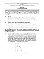
As illustrated in Figure 10.4b in the textbook, an increase in demand need not
always result in a higher price. Under the conditions portrayed in Figure 10.4b,
the monopolist supplies different quantities at the same price. Similarly, an
increase in supply facing the monopsonist need not always result in a higher price.
Suppose the average expenditure curve shifts from AE
1
to AE
2
, as illustrated in
Figure 10.1. With the shift in the average expenditure curve, the marginal
expenditure curve shifts from ME
1
to ME
2
. The ME
1
curve intersects the marginal
value curve (demand curve) at Q
1
, resulting in a price of P. When the AE curve
shifts, the ME
2

curve intersects the marginal value curve at Q
2
resulting in the same
price at P.
Price
Quantity
ME
1
AE
1
ME
2
AE
2
P
Q
1
Q
2
MV

Figure 10.1
2. Caterpillar Tractor, one of the largest producers of farm machinery in the world, has
hired you to advise them on pricing policy. One of the things the company would like to
know is how much a 5 percent increase in price is likely to reduce sales. What would you
need to know to help the company with this problem? Explain why these facts are
important.
As a large producer of farm equipment, Caterpillar Tractor has market power and
should consider the entire demand curve when choosing prices for its products. As
their advisor, you should focus on the determination of the elasticity of demand for

each product. There are three important factors to be considered. First, how
similar are the products offered by Caterpillar’s competitors? If they are close
138

Chapter 10: Market Power: Monopoly and Monopsony
substitutes, a small increase in price could induce customers to switch to the
competition. Secondly, what is the age of the existing stock of tractors? With an
older population of tractors, a 5 percent price increase induces a smaller drop in
demand. Finally, because farm tractors are a capital input in agricultural
production, what is the expected profitability of the agricultural sector? If farm
incomes are expected to fall, an increase in tractor prices induces a greater decline
in demand than one would estimate with information on only past sales and prices.
3. A monopolist firm faces a demand with constant elasticity of -2.0. It has a constant
marginal cost of $20 per unit and sets a price to maximize profit. If marginal cost should
increase by 25 percent, would the price charged also rise by 25 percent?
Yes. The monopolist’s pricing rule as a function of the elasticity of demand for
its product is:
(P - MC) 1
P
= -
E
d
1 +
E
d

or alternatively,
P =
MC
1

⎛
⎜
⎞
⎟
⎛
⎜
⎞
⎟
⎝ ⎠ ⎝ ⎠


In this example E
d
= -2.0, so 1/E
d
= -1/2; price should then be set so that:
P =
MC
1
2
⎛ ⎞
⎝ ⎠
=2MC

Therefore, if MC rises by 25 percent, then price will also rise by 25 percent.
When
MC = $20, P = $40. When MC rises to $20(1.25) = $25, the price rises to $50, a
25 percent increase.
4. A firm faces the following average revenue (demand) curve:
P = 120 - 0.02Q

where Q is weekly production and P is price, measured in cents per unit. The firm’s cost
function is given by C = 60Q + 25,000. Assume that the firm maximizes profits.
a. What is the level of production, price, and total profit per week?
The profit-maximizing output is found by setting marginal revenue equal to
marginal cost. Given a linear demand curve in inverse form, P = 120 - 0.02Q, we
know that the marginal revenue curve will have twice the slope of the demand
curve. Thus, the marginal revenue curve for the firm is MR = 120 - 0.04Q.
Marginal cost is simply the slope of the total cost curve. The slope of TC = 60Q +
25,000 is 60, so MC equals 60. Setting MR = MC to determine the profit-
maximizing quantity:
120 - 0.04Q = 60, or
Q = 1,500.
139

Chapter 10: Market Power: Monopoly and Monopsony
Substituting the profit-maximizing quantity into the inverse demand function to
determine the price:
P = 120 - (0.02)(1,500) = 90 cents.
Profit equals total revenue minus total cost:
π = (90)(1,500) - (25,000 + (60)(1,500)), or
π = $200 per week.
b. If the government decides to levy a tax of 14 cents per unit on this product, what will
be the new level of production, price, and profit?
Suppose initially that the consumers must pay the tax to the government. Since the
total price (including the tax) consumers would be willing to pay remains
unchanged, we know that the demand function is
P* + T = 120 - 0.02Q, or
P* = 120 - 0.02Q - T,
where P* is the price received by the suppliers. Because the tax increases the
price of each unit, total revenue for the monopolist decreases by TQ, and marginal

revenue, the revenue on each additional unit, decreases by T:
MR = 120 - 0.04Q - T
where T = 14 cents. To determine the profit-maximizing level of output with the
tax, equate marginal revenue with marginal cost:
120 - 0.04Q - 14 = 60, or
Q = 1,150 units.
Substituting Q into the demand function to determine price:
P* = 120 - (0.02)(1,150) - 14 = 83 cents.
Profit is total revenue minus total cost:
π
= 83
()
1,150
()
− 60
( )
1,150
( )
+ 25,000
( )
= 1450
cents, or
$14.50 per week.
Note: The price facing the consumer after the imposition of the tax is 97 cents.
The monopolist receives 83 cents. Therefore, the consumer and the monopolist
each pay 7 cents of the tax.
If the monopolist had to pay the tax instead of the consumer, we would arrive at the
same result. The monopolist’s cost function would then be
TC = 60Q + 25,000 + TQ = (60 + T)Q + 25,000.
The slope of the cost function is (60 + T), so MC = 60 + T. We set this MC to the

marginal revenue function from part (a):
120 - 0.04Q = 60 + 14, or
Q = 1,150.
Thus, it does not matter who sends the tax payment to the government. The
burden of the tax is reflected in the price of the good.
140

Chapter 10: Market Power: Monopoly and Monopsony
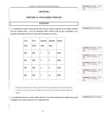
5. The following table shows the demand curve facing a monopolist who produces at a
constant marginal cost of $10.
Price Quantity
18 0
16 4
14 8
12 12
10 16
8 20
6 24
4 28
2 32
0 36
a. Calculate the firm’s marginal revenue curve.
To find the marginal revenue curve, we first derive the inverse demand curve. The
intercept of the inverse demand curve on the price axis is 18. The slope of the
inverse demand curve is the change in price divided by the change in quantity. For
example, a decrease in price from 18 to 16 yields an increase in quantity from 0 to
4. Therefore, the slope is
−
1
2

and the demand curve is
P =18−0.5Q.

The marginal revenue curve corresponding to a linear demand curve is a line with
the same intercept as the inverse demand curve and a slope that is twice as steep.
Therefore, the marginal revenue curve is
MR = 18 - Q.
b. What are the firm’s profit-maximizing output and price? What is its profit?
The monopolist’s maximizing output occurs where marginal revenue equals
marginal cost. Marginal cost is a constant $10. Setting MR equal to MC to
determine the profit-maximizing quantity:
18 - Q = 10, or Q = 8.
To find the profit-maximizing price, substitute this quantity into the demand
equation:
P = 18 − 0.5
( )
8
( )
= $14.

Total revenue is price times quantity:
TR = 14
( )
8
( )
= $112.

The profit of the firm is total revenue minus total cost, and total cost is equal to
average cost times the level of output produced. Since marginal cost is constant,
average variable cost is equal to marginal cost. Ignoring any fixed costs, total cost

is 10Q or 80, and profit is
112−80=$32.

c. What would the equilibrium price and quantity be in a competitive industry?
141

Chapter 10: Market Power: Monopoly and Monopsony
For a competitive industry, price would equal marginal cost at equilibrium.
Setting the expression for price equal to a marginal cost of 10:
18−0.5Q=10 ⇒Q=16⇒ P =10.

Note the increase in the equilibrium quantity compared to the monopoly solution.
d. What would the social gain be if this monopolist were forced to produce and price at
the competitive equilibrium? Who would gain and lose as a result?
The social gain arises from the elimination of deadweight loss. Deadweight loss in
this case is equal to the triangle above the constant marginal cost curve, below the
demand curve, and between the quantities 8 and 16, or numerically
(14-10)(16-8)(.5)=$16.
Consumers gain this deadweight loss plus the monopolist’s profit of $32. The
monopolist’s profits are reduced to zero, and the consumer surplus increases by
$48.
6. Suppose that an industry is characterized as follows:
C = 100 + 2Q
2
Firm total cost function
MC = 4Q Firm marginal cost function
P = 90 − 2Q Industry demand curve
MR = 90 − 4Q Industry marginal revenue curve.

a. If there is only one firm in the industry, find the monopoly price, quantity, and level

of profit.
If there is only one firm in the industry, then the firm will act like a monopolist
and produce at the point where marginal revenue is equal to marginal cost:
MC=4Q=90-4Q=MR
Q=11.25.
For a quantity of 11.25, the firm will charge a price P=90-2*11.25=$67.50. The
level of profit is $67.50*11.25-100-2*11.25*11.25=$406.25.


b. Find the price, quantity, and level of profit if the industry is competitive.
If the industry is competitive then price is equal to marginal cost, so that 90-
2Q=4Q, or Q=15. At a quantity of 15 price is equal to 60. The level of profit
is therefore 60*15-100-2*15*15=$350.
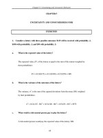
c. Graphically illustrate the demand curve, marginal revenue curve, marginal cost
curve, and average cost curve. Identify the difference between the profit level of
the monopoly and the profit level of the competitive industry in two different ways.
Verify that the two are numerically equivalent.
The graph below illustrates the demand curve, marginal revenue curve, and
marginal cost curve. The average cost curve hits the marginal cost curve at a
quantity of approximately 7, and is increasing thereafter (this is not shown in the
graph below). The profit that is lost by having the firm produce at the
142

Chapter 10: Market Power: Monopoly and Monopsony
competitive solution as compared to the monopoly solution is given by the
difference of the two profit levels as calculated in parts a and b above, or
$406.25-$350=$56.25. On the graph below, this difference is represented by the
lost profit area, which is the triangle below the marginal cost curve and above the
marginal revenue curve, between the quantities of 11.25 and 15. This is lost
profit because for each of these 3.75 units extra revenue earned was less than

extra cost incurred. This area can be calculated as 0.5*(60-45)*3.75+0.5*(45-
30)*3.75=$56.25. The second method of graphically illustrating the difference
in the two profit levels is to draw in the average cost curve and identify the two
profit boxes. The profit box is the difference between the total revenue box
(price times quantity) and the total cost box (average cost times quantity). The
monopolist will gain two areas and lose one area as compared to the competitive
firm, and these areas will sum to $56.25.
MC
MR
Dema nd
11.25 15
lost pr ofit
Q
P

7. Suppose a profit-maximizing monopolist is producing 800 units of output and is
charging a price of $40 per unit.
a. If the elasticity of demand for the product is –2, find the marginal cost of the last
unit produced.
Recall that the monopolist’s pricing rule as a function of the elasticity of demand
for its product is:
(P - M C) 1
P
= -
E
d
1 +
E
d

or alternatively,
P =
MC
1
⎛
⎜
⎞
⎟
⎛
⎜
⎞
⎟
⎝ ⎠ ⎝ ⎠
.

If we then plug in –2 for the elasticity and 40 for price we can solve to find
MC=20.
b. What is the firm’s percentage markup of price over marginal cost?
In percentage terms the mark-up is 50%, since marginal cost is 50% of price.
c. Suppose that the average cost of the last unit produced is $15 and the fixed cost is
$2000. Find the firm’s profit.
143

Chapter 10: Market Power: Monopoly and Monopsony
Total revenue is price times quantity, or $40*800=$32,000. Total cost is equal
to average cost times quantity, or $15*800=$12,000. Profit is then $20,000.
Producer surplus is profit plus fixed cost, or $22,000.
8. A firm has two factories for which costs are given by:
Factory # 1: C
1

Q
1
( )
= 10Q
1
2

Factory # 2: C
2
Q
2
( )
= 20Q
2
2

The firm faces the following demand curve:
P = 700 - 5Q
where Q is total output, i.e. Q = Q
1
+ Q
2
.
a. On a diagram, draw the marginal cost curves for the two factories, the average and
marginal revenue curves, and the total marginal cost curve (i.e., the marginal cost of
producing Q = Q
1
+ Q
2
). Indicate the profit-maximizing output for each factory,

total output, and price.
The average revenue curve is the demand curve,
P = 700 - 5Q.
For a linear demand curve, the marginal revenue curve has the same intercept as the
demand curve and a slope that is twice as steep:
MR = 700 - 10Q.
Next, determine the marginal cost of producing Q. To find the marginal cost of
production in Factory 1, take the first derivative of the cost function with respect to
Q:
dC
1
Q
1
( )
dQ
=20Q
1
.

Similarly, the marginal cost in Factory 2 is
dC
2
Q
2
( )
dQ
= 40Q
2
.

Rearranging the marginal cost equations in inverse form and horizontally summing
them, we obtain total marginal cost, MC
T
:
QQ Q
MC MC MC
T
=+= + =
12
12
20 40
3
40
,
or
MC
Q
T
=
40
3
.

Profit maximization occurs where MC
T
= MR. See Figure 10.8.a for the profit-
maximizing output for each factory, total output, and price.
144

Chapter 10: Market Power: Monopoly and Monopsony

Quantity
100
200
300
400
500
600
70 140
700
Price
800
P
M
MC
T
Q
T
MC
1
MC
2
Q
2
Q
1
MR
D

Figure 10.8.a
b. Calculate the values of Q

1
, Q
2
, Q, and P that maximize profit.
Calculate the total output that maximizes profit, i.e., Q such that MC
T
= MR:
40
3
700 10
Q
Q=−
, or Q = 30.
Next, observe the relationship between MC and MR for multiplant monopolies:
MR = MC
T
= MC
1
= MC
2
.
We know that at Q = 30, MR = 700 - (10)(30) = 400.
Therefore,
MC
1
= 400 = 20Q
1
, or Q
1
= 20 and

MC
2
= 400 = 40Q
2
, or Q
2
= 10.
To find the monopoly price, P
M
, substitute for Q in the demand equation:
P
M
= 700 - (5)(30), or
P
M
= 550.
c. Suppose labor costs increase in Factory 1 but not in Factory 2. How should the firm
adjust the following(i.e., raise, lower, or leave unchanged): Output in Factory 1?
Output in Factory 2? Total output? Price?
An increase in labor costs will lead to a horizontal shift to the left in MC
1
, causing
MC
T
to shift to the left as well (since it is the horizontal sum of MC
1
and MC
2
).
The new MC

T
curve intersects the MR curve at a lower quantity and higher
marginal revenue. At a higher level of marginal revenue, Q
2
is greater than at
145