Tài liệu Tracking and Kalman filtering made easy P8 ppt

8
GENERAL FORM FOR LINEAR
TIME-INVARIANT SYSTEM
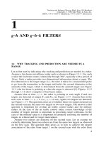
8.1 TARGET DYNAMICS DESCRIBED BY POLYNOMIAL AS A
FUNCTION OF TIME
8.1.1 Introduction
In Section 1.1 we defined the target dynamics model for target having a
constant velocity; see (1.1-1). A constant-velocity target is one whose trajectory
can be expressed by a polynomial of degree 1 in time, that is, d ¼ 1, in (5.9-1).
(In turn, the tracking filter need only be of degree 1, i.e., m ¼ 1.) Alternately, it
is a target for which the first derivative of its position versus time is a constant.
In Section 2.4 we rewrote the target dynamics model in matrix form using the
transition matrix È; see (2.4-1), (2.4-1a), and (2.4-1b). In Section 1.3 we gave
the target dynamics model for a constant accelerating target, that is, a target
whose trajectory follows a polynomial of degree 2 so that d ¼ 2; see (1.3-1).
We saw that this target also can be alternatively expressed in terms of the
transition equation as given by (2.4-1) with the state vector by (5.4-1) for m ¼ 2
and the transition matrix by (5.4-7); see also (2.9-9). In general, a target whose
dynamics are described exactly by a dth-degree polynomial given by (5.9-1) can
also have its target dynamics expressed by (2.4-1), which we repeat here for
convenience:
X
nþ1
¼ ÈX
n
where the state vector X
n
is now defined by (5.4-1) with m replaced by d and the
transition matrix is a generalized form of (5.4-7). Note that in this text d
represents the true degree of the target dynamics while m is the degree used by
252

Tracking and Kalman Filtering Made Easy. Eli Brookner
Copyright # 1998 John Wiley & Sons, Inc.
ISBNs: 0-471-18407-1 (Hardback); 0-471-22419-7 (Electronic)
the tracking filter to approximate the target dynamics. For the nonlinear
dynamics model case, discussed briefly in Section 5.11 when considering the
tracking of a satellite, d is the degree of the polynomial that approximates the
elliptical motion of the satellite to negligible error.
We shall now give three ways to derive the transition matrix of a target
whose dynamics are described by an arbitrary degree polynomial. In the process
we give three different methods for describing the target dynamics for a target
whose motion is given by a polynomial.
8.1.2 Linear Constant-Coefficient Differential Equation
Assume that the target dynamics is described exactly by the dth-degree
polynomial given by (5.9-1). Then its dth derivative equals a constant, that is,
D
d
xðtÞ¼const ð8:1-1Þ
while its ðd þ 1Þth derivative equals zero, that is,
D
dþ1
xðtÞ¼0 ð8:1-2Þ
As a result the class of all targets described by polynomials of degree d are also
described by the simple linear constant-coefficient differential equation given
by (8.1-2). Given (8.1-1) or (8.1-2) it is a straightforward manner to obtain the
target dynamics model form given by (1.1-1) or (2.4-1) to (2.4-1b) for the case
where d ¼ 1. Specifically, from (8.1-1) it follows that for this d ¼ 1 case
DxðtÞ¼
_
xðtÞ¼const ð8:1-3Þ
Thus

_
x
nþ1
¼
_
x
n
ð8:1-4Þ
Integrating this last equation yields
x
nþ1
¼ x
n
þ T
_
x
n
ð8:1-5Þ
Equations (8.1-4) and (8.1-5) are the target dynamics equations for the
constant-velocity target given by (1.1-1). Putting the above two equations in
matrix form yields (2.4-1) with the transition matrix È given by (2.4-1b), the
desired result. In a similar manner, starting with (8.1-1), one can derive the
form of the target dynamics for d ¼ 2 given by (1.3-1) with, in turn, È given
by (5.4-7). Thus for a target whose dynamics are given by a polynomial of
degree d, it is possible to obtain from the differential equation form for the
target dynamics given by (8.1-1) or (8.1-2), the transition matrix È by
integration.
TARGET DYNAMICS DESCRIBED BY POLYNOMIAL AS A FUNCTION OF TIME
253
8.1.3 Constant-Coefficient Linear Differential Vector Equation for

State Vector X(t)
A second method for obtaining the transition matrix È will now be developed.
As indicated above, in general, a target for which
D
d
xðtÞ¼const ð8:1-6Þ
can be expressed by
X
nþ1
¼ ÈX
n
ð8:1-7Þ
Assume a target described exactly by a polynomial of degree 2, that is, d ¼ 2.
Its continuous state vector can be written as
XðtÞ¼
xðtÞ
_
xðtÞ

xðtÞ
2
4
3
5
¼
xðtÞ
DxðtÞ
D
2
xðtÞ

2
4
3
5
ð8:1-8Þ
It is easily seen that this state vector satisfies the following constant-coefficient
linear differential vector equation:
DxðtÞ
D
2
xðtÞ
D
3
xðtÞ
2
4
3
5
¼
010
001
000
2
4
3
5
xðtÞ
DxðtÞ
D
2

xðtÞ
2
4
3
5
ð8:1-9Þ
or
d
dt
XðtÞ¼AXðtÞð8:1-10Þ
where
A ¼
010
001
000
2
4
3
5
ð8:1-10aÞ
The constant-coefficient linear differential vector equation given by (8.1-9), or
more generally by (8.1-10), is a very useful form that is often used in the
literature to describe the target dynamics of a time-invariant linear system. As
shown in the next section, it applies to a more general class of target dynamics
models than given by the polynomial trajectory. Let us proceed, however, for
the time being assuming that the target trajectory is described exactly by a
polynomial. We shall now show that the transition matrix È can be obtained
from the matrix A of (8.1-10).
254
GENERAL FORM FOR LINEAR TIME-INVARIANT SYSTEM

First express Xðt þ &Þ in a vector Taylor expansion as
Xðt þ &Þ¼XðtÞþ&DXðtÞþ
&
2
2!
D
2
XðtÞÁÁÁ
¼
X
1
¼0
&

 !
D
n
XðtÞð8:1-11Þ
From (8.1-10)
D

XðtÞ¼A

XðtÞð8:1-12Þ
Therefore (8.1-11) becomes
Xðt þ &Þ¼
X
1
¼0
ð&AÞ


 !
"#
XðtÞð8:1-13Þ
We know from simple algebra that
e
x
¼
X
1
¼0
x

 !
ð8:1-14Þ
Comparing (8.1-14) with (8.1-13), one would expect that
X
1
¼0
ð&AÞ

 !
¼ expð&AÞ¼Gð&AÞð8:1-15Þ
Although A is now a matrix, (8.1-15) indeed does hold with exp ¼ e being to a
matrix power being defined by (8.1-15). Moreover, the exponent function
GðAÞ has the properties one expects for an exponential. These are [5, p. 95]
Gð&
1
AÞGð&
2

AÞ¼G½ð&
1
þ &
2
ÞAð8:1-16Þ
½Gð&
1
AÞ
k
¼ Gðk&
1
AÞð8:1-17Þ
d
d&
Gð&AÞ¼Gð&AÞA ð8:1-18Þ
We can thus rewrite (8.1-13) as
Xðt þ &Þ¼expð&AÞXðtÞð8:1-19Þ
Comparing (8.1-19) with (8.1-7), we see immediately that the transition matrix
is
Èð&Þ¼ expð&AÞð8:1-20Þ
TARGET DYNAMICS DESCRIBED BY POLYNOMIAL AS A FUNCTION OF TIME
255
for the target whose dynamics are described by the constant-coefficient
linear vector differential equation given by (8.1-10). Substituting (8.1-20) into
(8.1-19) yields
Xðt
n
þ &Þ¼Èð&ÞXðt
n
Þð8:1-21Þ

Also from (8.1-15), and (8.1-20) it follows
Èð&Þ¼I þ &A þ
&
2
2!
A
2
þ
&
3
3!
A
3
þÁÁÁ ð8:1-22Þ
From (8.1-17) it follows that
ðexp &AÞ
k
¼ exp k&A ð8:1-23Þ
Therefore
½Èð&Þ
k
¼ Èðk&Þð8:1-24Þ
By way of example, assume a target having a polynomial trajectory of degree
d ¼ 2. From (8.1-10a) we have A. Substituting this value for A into (8.1-22) and
letting & ¼ T yields (5.4-7), the transition matrix for the constant-accelerating
target as desired.
8.1.4 Constant-Coefficient Linear Differential Vector Equation for
Transition Matrix È
A third useful alternate way for obtaining È is now developed [5. pp. 96–97].
First, from (8.1-21) we have

Xð&Þ¼Èð&ÞXð0Þð8:1-25Þ
Differentiating with respect to & yields
d
d&
Èð&Þ

Xð0Þ¼
d
d&
Xð&Þð8:1-26Þ
The differentiation of a matrix by & consists of differentiating each element
of the matrix with respect to &. Applying (8.1-10) and (8.1-25) to (8.1-26)
yields
d
d&
Èð&Þ

Xð0Þ¼AXð&Þ
¼ AÈð&ÞXð0Þð8:1-27Þ
256
GENERAL FORM FOR LINEAR TIME-INVARIANT SYSTEM