Tài liệu Các mạng UTMS và công nghệ truy cập vô tuyến P7 docx
Bạn đang xem bản rút gọn của tài liệu. Xem và tải ngay bản đầy đủ của tài liệu tại đây (1022.58 KB, 53 trang )
The UMTS Network and Radio Access Technology: Air Interface Techniques for Future Mobile Systems
Jonathan P. Castro
Copyright © 2001 John Wiley & Sons Ltd
Print ISBN 0-471-81375-3 Online ISBN 0-470-84172-9
D
EPLOYING
3G N
ETWORKS
7.1 B
ACKGROUND
Logically deploying 3G networks implies dimensioning and implementing corresponding
elements within a geographical area, where an operator would desire to offer advanced
mobile communications services, e.g. voice, mobile Internet, video-telephony, etc.
In the preceding chapters we have outlined the service requirements and technical speci-
fications of the UMTS solution. In this chapter we aim to describe the application of the
proposed solutions and go through the process of designing a network to provide UMTS
services.
Before describing the results of a field study with reference-parameters based on real
scenarios, we provide the necessary principles for dimensioning and implementing a 3G
network using UMTS technology. We then present results of dimensioning and intro-
duce the functional capabilities of the selected elements.
7.2 N
ETWORK
D
IMENSIONING
P
RINCIPLES
Figure 7.1 identifies non-exhaustively the major areas to dimension a 3G network. It
summarizes the essential tasks to obtain the necessary count of elements for implemen-
tation and network deployment.
9vrvvtÃhx
Ã
8hhpvÃhq
Ã
prhtrÃphypyhv
Ã
IrxÃ
rshprÃ
rhrrÃhqÃ
rhyhvÃ
ShqvÃrxÃ
hvvÃ
qvrvvtÃ
8rÃrxÃ
hvvÃ
qvrvvtÃ
ShqvÃhqÃ8IÃ
hvvÃ
vrthvÃ
IrxÃ
vvhvÃ
&RYHUDJH
Ã
ÈÃsÃhhvyhiyrÃrhvÃ
ÃrtvÃ
UhvvÃhrh)Ã
Vih
ÃiihÃhyÃ
rpÃ
ShqvÃhthv)Ã
HhpÃvpÃvpÃ
ÃuvrhpuvphypryyÃ
rvrÃ
8hhpvÃyrry)Ã
UrÃsÃhssvpÃhqÃ
rvprÃ
RhyvÃsÃrvpr)Ã
7ypxvtÃihivyvÃ
rvprÃhhvyhivyvÃ
IrxÃrshpr)
Ã
@ssvpvrpÃhqrssÃ
IirÃsÃSI8Ã
prrÃ
IirÃsÃihrÃ
hvÃ7TÃvrÃ
7TÃpsvthvÃ
vÃ
8uvprÃsÃhqvÃ
rprÃhhtrrÃ
SSHÃhytvuÃ
8hhpvÃhqÃprhtrÃ
rvsvphvÃ
RhyvÃsÃrvprÃ
ryrpvÃ
DqrvsvphvÃsÃxrÃ
SSHÃhhrrÃ
UhvvÃrxÃ
phhpvÃ
DÃsÃrvrr
Ã
Sry
Ã
Figure 7.1 Essential network dimensioning tasks.
To simplify the whole process we group the dimensioning tasks into four key iterative
actions, i.e.
248 The UMTS Network and Radio Access Technology
radio coverage and traffic flow identification;
system dimensioning;
network configuration and verification (i.e. radio, core, transmission);
implementation and deployment.
In the first action, radio coverage depends on both propagation environment, (i.e. ser-
vice population areas) and the traffic flow expected. Through a computerized process
and classical optimization, the main output consists of the identification of sites for BS
(or node B) location. The latter will depend on the projected service strategy and the BS
range and capacity. The service strategy will take into account the traffic flow generated
based on the subscriber profiles of service utilization levels and population densities.
The radio coverage task will include or use the multi-path channel models, and refer-
ence service rates illustrated in Chapter 2.
System dimensioning involves the optimization of coverage and capacity based on mac-
rocells and microcells in densely populated areas. It aims to take into account the asym-
metry of traffic in the UL and DL and includes in the optimization the TDD mode to
maximize capacity and flexibility in micro- and picocells.
Network configuration and verification consolidates the coverage and site location ex-
ercise by starting a process for the integrated solution of radio and core elements. Based
on the capacity and service target requirements, the 3G system architecture is set for the
node Bs and CS and PS elements in the core network side. It also looks at the impact on
the transmission subsystem.
Implementation and deployment completes the 3G-network design process by realizing
the projected site locations, service target requirements and time to service. It takes into
account the solution adopted for the network deployment, e.g. sharing sites with exist-
ing 2G BSs and evolution of CN elements, or a complete new overlay network on the
top of the existing 2G system. It may also apply to a totally green field network, i.e. a
new deployment. It will also take into account the hierarchy of the network, i.e. the
macro- and microlayers where applicable.
When deploying in the macrocell environment primarily with the FDD mode or
WCDMA technology, the implementation will take into account the coverage depend-
ency on the transmission rates and technology availability in terms of antenna configu-
ration and interference minimizing features. Thus, the four actions or steps outlined
above do have an iterative process.
7.2.1 Coverage and Capacity Trade-off in the FDD Mode
From the practical side as mentioned in earlier chapters and Section 7.4 of this chapter,
in the FDD mode, which uses WCDMA techniques, the interference increases with the
number of active users, thereby limiting capacity. Within this soft limitation, the system
quality decreases continuously until service performance degrades to an intolerable
state. This state leads to the breathing cells phenomenon, i.e. when user numbers gets
too high, the quality of users at the cell-edge degrades rapidly to the point to drop the
link or the call. Such event implies that cell radio coverage shrinks. On the other hand,
when call drops occur, interference decreases for the remaining users and cell area cov-
Deploying 3G Networks 249
erage grows again. This is what we call the trade off between capacity and coverage in
the FDD mode.
Cell coverage and capacity thus depend on the received bit energy to total noise plus
interference ratio E
b
/(N
0
+ I
0
) on each cell part for the DL and in the BS for the UL.
This means that any parameter, which affects the signal level and/or the interference
1
, or
reduces the E
b
/(N
0
+ I
0
) requirements
2
, has impact on cell coverage and capacity, as
well as on the overall system.
7.2.1.1 Soft Handover and Orthogonality
We described soft handover in Chapter 4 from the design side; here we look at it from
the performance and dimensioning side. In this context, a MS performs handover when
the signal strength of a neighbouring cell exceeds the signal strength of the current cell
with a given threshold. In soft handover position, a MS connects to more than one BS
simultaneously. Thus, the FDD mode uses soft handover
3
to minimize interference into
neighbouring cells and thereby improve performance through macro diversity, i.e. we
combine all the paths together to get a better signal quality. We also reduce power
originating from two or more BSs to reach the same mobile’s E
b
/N
0
requirement while
we combine the paths.
We separate the information signal of different users by assigning to each one a differ-
ent broadband and time limited, user specific carrier signal derived from orthogonal
code sequences (e.g. OVSF codes). When completely orthogonal
4
, we can perfectly
separate synchronously transmitted and received signals. However, this does not occur
in the UL for example, due to different propagation paths, i.e. different distances with
different time delays. In the DL even if all signals originate from a single point and the
parallel code channels can be synchronized there is still not perfect signal separation. As
a result, we cannot maintain complete orthogonality due to multipath propagation, and
we have to use orthogonality compensation factors as noted in Chapter 2.
7.3 P
ARAMETERS FOR
M
ULTISERVICE
T
RAFFIC
While some earlier
5
2G mobile systems measure network quality mainly for one ser-
vice, e.g. speech, UMTS has many different bearer services with varying quality re-
quirements. We characterize these differing services by parameters such as the bit rate,
the maximal delay, connection symmetry, and tolerable maximum BER. As result to
accurately dimension or design a network for multiple services, we need to use different
traffic models and settings. We have to plan the BS numbers to handle the expected
service mix. The multiple set of services will have different impact on capacity and
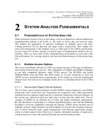
coverage. For example, user bit rate will have large impact on coverage as illustrated in
_______
1
Interference = intracell interference and intercell interference.
2
Interference here implies intracell interference and intercell interference.
3
Softer handover is a soft handover between two sectors of a site.
4
Two function orthogonality, e.g. g(t) and s(t), occurs when their cross-correlation functions equal zero.
5
Today GSM evolved to a more than just speech network, it does also GPRS and HSCSD.
250 The UMTS Network and Radio Access Technology
Figure 7.2. On the other hand, we can often adjust all services to the same cell range by
individually adjusting the emitted power of each service.
TrrpuÃhqÃGÃ9hhÃShrHrqvÃ9hhÃShr
CvtuÃ9hhÃShr
Figure 7.2 Transmission rates and coverage.
7.3.1 Circuit and Packet Switched Services
When dimensioning a 3G network in the FDD mode, e.g. the number of concurrent
channels derived to cope with the different service requirements becomes the main in-
put of the link budget analysis. Thus, if we have to manage traffic beyond a cell loading
of 30%, any small load variation will have direct impact on the cell radius. We then
have to achieve a dimensioning to meet the peak traffic during the busy hour in order to
obtain a stable network. This stability will depend on how we treat the different types of
service, i.e. Real Time (RT) or Circuit Switched and Non Real Time (NRT) or packet
switched types.
7.3.1.1 Circuit Switched (CS)
To dimension capacity for CS services we can follow the classical approach, i.e. given
the offered load (Erlangs) and the blocking rate, we derive from the traffic assumptions
the offered traffic at the busy hour per cell (Erlang). Here we would assume the cell
radius gets optimized iteratively with the link budget. Then, from Erlang B table we
would determine the number of concurrent channels required during the busy hour for a
given blocking rate.
Although the traditional solution may allow us to estimate CS capacity easily, it may
also over dimension the required number of channels. Thus, it seems imperative that we
use the multi-service Erlang B formulation and pool the resources for better availability
on demand. This implies that we offer the CS channels depending on the required num-
ber, e.g. if one service requires 2 channels and the other 10, both can benefit from the
pool, which may contain 20 channels. The latter would also imply that we could use
different blocking rates for each service. For example, voice calls can tolerate degrada-
tion better than video calls.
7.3.1.2 Packet Switched Services
As in the CS, although with more sophistication, we also need to estimate the number of
concurrent channels required for PS traffic. This number of channels will correspond to
Deploying 3G Networks 251
the peak traffic during a Busy Hour (BH), which as in the CS, we determine also from
the traffic assumptions of the offered load during the busy hour per cell expressed in
kbits. In general, we treat each service independently to meet the different grade of ser-
vice or asymmetry required.
We calculate the number of PS service channels by accounting a duration window cor-
responding to an acceptable delay (e.g. d
§
–07 s) for a given service. From the prin-
ciples outlined in Chapter 2, we can illustrate the calculation for WWW application
6
as
follows.
We take 384 kps service with packet length
z
= 480 bytes. From the total BH traffic for
a given reference area we calculate the mean offered data rate m in kbps. Translating
this into a mean packet arrival p rate, i.e. p = (m
d)/
z
.. Then assuming a Poisson
packet arrival distribution for all users, with a mean p, we obtain the probability density
function (PDF), as well as the cumulative density function (CDF). Figure 7.3 illustrates
the peak packet arrival rate h at 95% time probability [7].
9yvxÃÃQvÃ9vvivÃÃ2Ã$Ã 2 &
'
%
!#
"!
#
#'
$%
%#
&!
'
''
(%
#
!
"
#
$
%
&
'
(
!
"
#
$
%
&
'
(
!
!
!!
!"
!#
!$
!%
!&
!'
!(
"
"
"!
xÃ6vhyÃvÃUÃrp
QxÃ6vhyÃvÃÃrpÃÃbQ9AdÃ
$
$
!
!$
"
"$
#
#$
$
$$
%
%$
&
&$
'
'$
(
($
$
QxÃQ9A
89A
Figure 7.3 Peak arrival rate.
Utilizing the upper 95% time probability of the packet arrival rate (Figure 7.3) and ap-
plying the typical packet length we translated back into kbps. We then calculate the
number of channels (ch) dividing by the service bearer rate r, i.e. ch = h (kbps)/r. We
can summarize the process as: Chs = (1/Serv Rate) × (1/Serv Delay) × CDFp{(m/Serv
delay ×
z
),95%), where CDFp(x,y) corresponds to the point of probability on the CDF
associated with Poisson’s law of mean x, and where m represents the mean offered data
rate in kbps. We should note here that this process can be inefficient with low traffic in
the cell, resulting in over-dimensioning for PS services. Thus, other types of distribution
should also be considered.
_______
6
For example e-commerce, on line banking, file transfer, information DB access, etc.
252 The UMTS Network and Radio Access Technology
7.4 E
STABLISHING
S
ERVICE
M
ODELS
Before deploying new elements in a mobile telecommunications network, whether it is
an existing system based on 2nd generation (2G) technology like GSM, or a new one
like UMTS, we will need a projection for the potential number of subscribers. In this
chapter, we consider a field study to extrapolate some subscriber numbers from two
growth forecast
7
assumptions. Although these projections will not necessarily apply to a
particular deployment scenario, it will serve to illustrate network dimensioning based on
the split of voice only and combined (voice + data) services.
In Table 7.1 we illustrate estimations for a 10-year period where 2G values correspond
primarily to GSM voice services and 3G values to data starting with GPRS in the 1st
2 years. Thereafter, full multimedia services expand rapidly at the introduction of
UMTS in existing GSM networks. A major breaking point occurs around 2005 with
high predominance of 3G type services.
Table 7.1 Subscriber Growth Within a 10-year Period (in 1000s)
Subscribers
Year: 2000 2001 2002 2003 2004 2005 2006 2007 2008 2009
2G 750 1000 900 600 400 300 200 150 100 50
3G 0 0 300 700 1000 1200 1400 1500 1600 1700
Total 750 1000 1200 1300 1400 1500 1600 1650 1700 1750
In Table 7.2 we illustrate the subscriber growth beginning in 2002 when penetration of
data has already reached about 30% of the total traffic. Here we assume that GPRS car-
rying wireless IP type services has grown to non-negligible levels right before the intro-
duction of UMTS. Despite the stretch to a 15-year period, 2005 stands again as the
breaking point towards full predominance of multimedia services. Nonetheless, as in the
projections of the 10-year period, voice only services will remain a good 25% of all
traffic.
Table 7.2 Subscriber Growth Within a 15-year Period (in 1000s)
Ã
Subscribers
Year: 2002 2003 2004 2005 2007 2009 2011 2013 2015 2017
Voice 900 600 400 300 150 100 50 0 0 0
Voice
+ data
300 700 1000 1200 1450 1550 1650 1750 1800 1850
Total 1200 1300 1400 1500 1600 1650 1700 1750 1800 1850
After 2005 in both cases the subscriber growth appears low. This can reflect the fact
that the overall penetration of mobile services in the region begins to reach its limits or
that the market share between operators starts to stabilize. Thus, for all practical pur-
poses, in particular for the network dimensioning exercise in this field study, we con-
sider primarily the data from 2002 to 2005 from Table 7.2.
_______
7
The forecast has harmonized numbers, which do not apply to any operator or service provider in particular.
Deploying 3G Networks 253
7.5 P
ROJECTING
C
APACITY
N
EEDS
Based on the preceding section dimensioning in this field study would then begin for
about 1.5 million subscribers all using either voice only or multimedia services. The
proportion will depend on the business strategy and the type of service products offered.
Business strategy will have a strong relationship with the market segment addressed and
the penetration of the type of services proposed. If we take Switzerland, for example,
penetration of mobile services will reach 60% in all segments by the time we complete
this writing. Clearly, voice appears as the predominant service, although data through
SMS and HSCSD and early GPRS may grow. This means that the market for multime-
dia services remains quite open even up to 100%. Thus, following a pragmatic ap-
proach, network dimensioning and capacity projections will imperatively be done for
multimedia services addressing all segments.
Now for all practical purposes we identify three main segments, i.e. business, residen-
tial, and mass market (see Chapter 6). The traffic distribution among these segments
will depend on the subscriber demand, operator’s service
8
offer, and qualitative think-
ing. Nevertheless, looking at the data in Table 7.1 and Table 7.2, about 70% of the mar-
ket stands open for multimedia type services. If we distribute the latter as 40% mass
market and 15% business and residential, respectively; then dimensioning should follow
conventional wisdom.
Conventional wisdom may tell us that residential and business segments will tend to use
larger transmission rates (e.g. 384 kbps) in suburban and urban areas, while mass-
market subscribers will use medium rates services (144 kbps) from everywhere.
7.6 C
ELLULAR
C
OVERAGE
P
LANNING
I
SSUES
Before discussing the fundamental parameters, assumptions and planning methodology,
we select a region with a typical subscriber population and complex geographical area
for cellular planning, e.g. mountainous landscape with large canyons and valleys, as
well as hilly cities.
7.6.1 The Coverage Concept
As illustrated in Figure 7.4 the ideal UMTS coverage concerns all types of environ-
ments, i.e. in buildings (picocells), urban (microcells), suburban (macrocells), and
global (global cells). However, at this time we cover mainly picocells to macrocells.
While FDD coverage here may apply primarily
9
to macrocells, the TDD solution ap-
plies more to pico- and microcells. Figure 7.5 shows an option for combining the UTRA
technologies for maximum coverage.
_______
8
The operator’s initiative and creativity on new services offering product packages and a business approach
will make a large difference. It will not depend only on Internet traffic.
9
The FDD also applies to microcells, and it is not only for use in picocells.
Deploying 3G Networks 255
this field study, we assume that TDD can apply to dense urban areas and concentrate on
macrocell dimensioning for FDD or WCDMA.
7.6.2 Radio Network Parameter Assumptions
Figure 7.6 illustrates the coverage within a geographical area. Logically, an operator or
service provider will aim to have 99% coverage for the populated area while maximiz-
ing the geographical coverage. On the other hand, the penetration of UMTS at the intro-
duction will not necessarily include all populated
11
environments. Thus, starting in the
main cities and suburban areas, 3G network coverage can progress in three phases, i.e.
50%, 75 (80)%, and 99%. For business strategic reasons within a region, e.g. it would
be expedient to cover also major vacation centres even if these areas do not have per-
manent population, but transitory during a quarter of the year. Which means a sound
business case for the introduction of UMTS would start with more than just 50% cover-
age of the populated area.
With the assumptions above, in the following we outline key issues when designing a
macrocellular network based on the FDD mode or WCDMA.
Figure 7.6 Population coverage example.
Figure 7.7 illustrates the conversion of population density to area coverage, where 50%
of the population corresponds to about 10% of the coverage area. Thus, we can tailor
coverage depending on strategy or demand once basic coverage has been achieved.
Table 7.3 illustrates the morphology distribution of the 50 and 75% population cover-
age. It indicates area coverage proportion in km
2
of the different service environments,
i.e. dense urban (DU), urban (U), commercial/industrial (CI), suburban (SU), forest
(FO), open (OP). It also indicates the service area proportions in % of the total area cor-
responding to the 50 or 75% population density. These proportions serve as the points
of reference to establish the number of subscribers per service area and plan accordingly
for the number of sites or cells required for each service environment. It will also allow
estimation of RF unit number according to the number of sectors per site.
_______
11
Regulators in some countries are demanding only 50% initial coverage.
256 The UMTS Network and Radio Access Technology
Ã
È
È
!È
"È
#È
$È
%È
&È
'È
(È
È
È
È
!È
"È
#È
$È
%È
&È
'È
(È
È
QPQÈ
Figure 7.7 Population density conversion to area coverage.
Table 7.3 Morphology Distribution of the Population Density
Coverage area 50% POP 75% POP
Total size (km
2
) 4067.00 6741.00
Morphology distribution (km
2
)
Dense urban 2.33 2.37
Urban 9.90 10.60
Commercial/industrial 101.00 138.00
Suburban 387.00 617.00
Forest 1270.00 1961.00
Open 2297.00 4012.00
Morphology distribution
Dense urban (%) 0.06 0.04
Urban (%) 0.24 0.16
Commercial/industrial (%) 2.48 2.05
Suburban (%) 9.52 9.15
Forest (%) 31.23 29.09
Open (%) 56.48 59.52
Table 7.4 illustrates the service quality assumptions for projected radio bearer services
in UMTS. The transmission rates or bearers corresponding to the service environments
represent the most common services. On the other hand, we do not necessarily exclude
speech, LCD 384, LCD 2048, and UDD 2048. For example, voice service may have the
following assumptions: Adaptive Multi Rate (AMR) codec with a bit-rate of 12.2 kbits/
s and with 50% voice activity factor. We can also assume 20 mE/subs with the follow-
ing average holding times per subscriber:
holding time of a mobile originated call 75 s
holding time of a mobile terminated call 90 s
Deploying 3G Networks 257
The traffic distribution is estimated:
proportion of call attempts that is mobile originated 0.60
and mobile terminated 0.40
Table 7.4 Service Quality Requirements
Area/bearer service LCD 64 LCD 144 UDD 64 UDD 144 UDD 384
Dense urban Indoor
LCP 95%
Indoor
LCP 95%
Indoor
LCP 95%
Indoor
LCP 95%
Indoor
LCP 95%
Urban Indoor
LCP 95%
Indoor
LCP 95%
Indoor
LCP 95%
Indoor
LCP 95%
Indoor
LCP 95%
Commercial/industrial Indoor
LCP 95%
Indoor
LCP 95%
Indoor
LCP 95%
Indoor
LCP 95%
Indoor
LCP 90%
Suburban Indoor
LCP 90%
Indoor
LCP 90%
Indoor
LCP 90%
Indoor
LCP 90%
Forest In-car LCP
90%
In-car LCP
90%
In-car LCP
90%
In-car LCP
90%
Open In-car LCP
90%
In-car LCP
90%
In-car LCP
90%
In-car LCP
90%
LCD 384 and LCD 2048 can be considered for indoor transmission with LCP 95%. The
number of subscriber with these rates in each cell will not exceed a couple of users. The
traffic data example illustrated in Table 7.5 shows a possible distribution of the different
type of bearer services. Notice it does not include voice services.
Table 7.5 Traffic Data Example for 50 and 75% Population Coverage
Area
DU U IND SU FO OP
Active subscribers at 50% popula-
tion coverage
6000 21000 80000 265000 70000 30800
Active subscribers at 75% popula-
tion coverage
7000 22000 110000 350000 110000 401000
Busy hour traffic/subscriber UL
Bearer UDD64 (kbit/s) 0.079 0.079 0.079 0.08 0.08 0.08
Bearer UDD144 (kbit/s) 0.060 0.060 0.060 0.07 0.07 0.07
Bearer UDD384 (kbit/s) 0.015 0.015 0.015
Bearer LCD64 (mErl) 0.50 0.50 0.50 0.50 0.50 0.50
Bearer LCD144 (mErl) 0.25 0.25 0.25 0.25 0.25 0.25
Busy hour traffic/subscriber DL
Bearer UDD64 (kbit/s) 0.120 0.120 0.120 0.15 0.15 0.15
Bearer UDD144 (kbit/s) 0.18 0.18 0.18 0.24 0.24 0.24
Bearer UDD384 (kbit/s) 0.08 0.08 0.08
Bearer LCD64 (mErl) 0.50 0.50 0.50 0.50 0.50 0.50
Bearer LCD144 (mErl) 0.25 0.25 0.25 0.25 0.25 0.25
The traffic data, i.e. Unrestricted Delay Data (UDD) and Low delay Circuit Switch Data
(LCD) for the different environments (Dense Urban (DU), Urban (U), Industrial (IND),
Suburban (SU), Forest (FO), and Open (OP)), represent the possible traffic flow in the
3G network. We provide them here only as reference to make realistic projections. No-
tice that the traffic in the DL is higher than in the UL due to the fact the users download
258 The UMTS Network and Radio Access Technology
more information than they upload. We can also see that a good part of the subscriber
base remains in the open areas in this particular density distribution.
Consolidating 3G BS areas will vary from region to region. Some regions have already
strict regulations for the implementation of sites as well as high costs in dense areas.
This means that site acquisition will exceed the minimum requirements. Thus, Table 7.5
shows the necessary margins projected for subscriber growth assuming that sites can be
available within a short term. The turnaround to prepare sites to increase coverage and
capacity may not necessarily match a rapid subscriber growth. If we apply 50% of the
population coverage to the 1st case and 75% to the 2nd case, we then have about 750K
UMTS subscribers for the initial phase and about 1000K for the latter. This means we
dimension the 3G network initially with enough margin for growth towards the latter
phase where the subscriber base approaches the predicted numbers for 2005 in Table
7.1 when adding the 2G subscribers, i.e.
§.VXEVFULEHUV
7.6.3 Circuit Switched Data Calls Assumptions
From [1] for 64 kbps UDI we, assumed that 25% of the UMTS subscribers will also be
CS data subscribers. We also assume that 50% of the calls will be UL + DL, 25% of the
calls will be UL only and 25% of the calls will be DL only. This means, that one call
will occupy two channels (one for DL and one for UL) but with a 75% usage each.
CS data users may use multimedia with the following traffic mix:
1 data call per 24 h, with a duration of 30 min. We assume that 50% of these calls
occur during busy hour (BHCA=0.5); 3% of the CS data users use this service;
1 data call per 3 h, with a duration of 5 min. It is assumed that 67% of these calls
are done during busy hour (BHCA=0.67); 6% of the CS data users use this service.
CS Data users may use other UDI services with the following traffic:
1 data call per 3 h, with a duration of 5 min. It is assumed that 67% of these calls
are done during busy hour (BHCA=0.67); 3% of the CS data users use this service.
7.6.4 Packet Switched Applications
Packet data traffic will have different requirements on delays, packet loss, etc. The rec-
ommended classes include streaming, conversational, interactive and background. On this
basis Table 7.6 illustrates the traffic mix of users and total traffic that may be applied.
Table 7.6 Packet Traffic Mix
Scenario
% Users % Traffic Traffic BH (kbytes) Traffic classes
DL UL Total
Background 59 21 49 16 65
Interactive 156* 39 110 20 130
Streaming 4 18 50 10 60
Conversational 5 22 38 38 76
Total 100 247 84 331
* Note that each subscriber may use several applications.
Deploying 3G Networks 259
7.6.5 Characteristic of CDMA Cells
The factors affecting CDMA cell size, capacity, and co-channel parameters in the for-
ward and reverse links include same cell interference and other cell interference. These
events also have impact on the link power budgets.
7.6.5.1 Theoretical Capacity
Here we look at capacity from the user interference side. To illustrate a basic case, we
use the link reference parameter, i.e. E
b
/N
o
, or energy per pit per noise power density,
which later will apply to the link budget frame work.
Picking it up from equation (2.6), we consider the generic reverse-link capacity in
CDMA
12
as the limiting factor. Thus, assuming perfect power control for this instance,
the received powers from all mobiles users are the same. Then
6
10
=
-
where M is the total number of active users in a given band, and where the total inter-
ference power in the band equals the sum of powers of single users. Now equating the
energy per bit to the average modulating signal power we defined
E
6
(67
5
==
where S is the average modulating signal power, T is bit time duration, and R is the bit
rate, i.e. 1/T. Then, incorporating the noise power density N
o
, which is the total noise
power N divided by the bandwidth B (i.e. N
o
= N/B), we get
()
E
R
( 6% %
1150 5
==
-
Solving for M yields
()
()
ER
% 5
0
( 1
-=
DQGIRUODUJH0ZHJHW
()
()()
S
*
%5
0
( 1(1
==
where G
p
corresponds to the system processing gain defined in equation (2.3), and M
defines the number of projected users in a single CDMA cell with omnidirectional an-
tenna without interference from neighbouring cells users transmitting continuously.
7.6.5.2 The Cell Loading Effect
Since in real 3G mobile networks there always exists more than one cell and more than
one sector, we need to introduce a loading effect due to interference from neighbouring
cells as follows:
_______
12
Mainly in rural areas; in urban area the downlink may/will become the limiting factor.
260 The UMTS Network and Radio Access Technology
()
E
R
(%
105
ËÛ
=
ÌÜ
-+b
ÍÝ
where is the loading factor (ranging from 0 to 100%) as introduced in equation (2.29).
Typical
values will range from 45 to 50%. The inverse of as (1 +
has often been
defined as the frequency re-use factor, i.e. F = 1/(1 +
). The ideal single cell CDMA
value of F = 1 (i.e.
= 0) decreases as the loading of multi-cell environments increase.
Sectorization can decrease interference from other users in other cells. Thus, instead of
deploying only omnidirectional antennas with 360º a majority (if not) all sites can bear
at least three sectors (e.g. 120º), and allow thereby the sectorized antenna to reject inter-
ference from users outside its antenna pattern. Such an event will decrease the loading
effect and int
URGXFHDVHFWRUL]DWLRQJDLQ ZKLFKFDQEHH[SUHVVHGDV
()
()
()
()
*
*
G
G
,
$
,
$
p
p
l=
ËÛ
q
ÌÜ
ÌÜ
ÍÝ
×
×
where A
G
(0) is the peak antenna gain occurring generally at the bore sight (i.e.
A
G
is the horizontal antenna pattern of the sector antenna; I
represents the received
interference power from users of other cells as a function of
.
,QSUDFWLFH IRUD
three sector configuration and about 5 for a six sector one. Then, incorporating the sec-
torization gain in the loading effect, we get:
()
E
R
(%
105
ËÛ
=l
ÌÜ
-+b
ÍÝ
Initially for the single cell case, we have assumed continuous transmission. However,
this does not occur for voice and some multimedia services; although it does for data.
Thus, we will now introduce an activity factor 1/
to reflect this event in the UL loading
effect. Then, we get
()
E
R
(%
105
ËÛ
ËÛ
=l
ÌÜ
ÌÜ
-+bn
ÍÝ
ÍÝ
where may range from 40 to 50% for voice and 1% for data. Therefore, the value of
reduces the overall interference of the UL loading effect equation.
For the downlink (DL) we need an additional parameter
to reflect the orthogonality of
the transmission. Thus empirically, we can express it as:
()
E
R
(%
105
ËÛ
ËÛ
=l
ÌÜ
ÌÜ
--e+bn
ÍÝ
ÍÝ
Deploying 3G Networks 261
7.6.6 Link Budgets
A link budget aims to provide the steps to calculate the ratio of the received bit energy
to thermal noise (i.e. E
b
/N
o
) and the interference density I
o
. It considers transmit power,
transmit and receive antenna gains, channel capacity factors, propagation environment,
and receiver noise figure.
Based on the channel models introduced in Chapter 2 we present the background for
link budgets. Following the guidelines from Ref. [3] the formulation assumes that path
loss formulas help to determine the maximum range and the coverage area. We also
assume that in the case of hexagonal deployment of sectored cells, the area covered by
one sector is:
5
6
ËÛ
=
ÌÜ
ÍÝ
where R is the range obtained in the link budget. This implies that we use hexagonal
sectors with base stations placed in the corners of the hexagons. Coverage analysis can
thus apply to tri-sectored antennas for macrocells and with omnidirectional antennas for
microcell and picocell coverage.
Before describing the actual reference parameters for the link budgets in Table 7.7, in
the following we provide a generic background of the analysis steps for the forward and
reverse links.
7.6.6.1 The Forward Link
Applying the logic for the traffic channels analysis in Ref. [2], to the Dedicated Physical
Control Channel (DPCCH) and Dedicated Physical Data Channel (DPDCH) we can
formulate a generic E
b
/N
o
for the forward link in a multi-cellular environment.
Starting from a single cell with a single mobile station (MS),
E RR*
REQ
(3/$
*
1,,1
=
++
where P
o
is the BS sector traffic channel ERP in the direction of the MS within a given
antenna pattern with its angle
o
, L
o
equal to the path loss from the home BS in the di-
rection of
o
within a given distance, A
G
is the receive antenna gain the MS, I
n
is equals
to the interference power received at the MS from non-CDMA origins, N is the thermal
noise power, G is the processing gain, and I
b
can be defined as:
E R*
,3/$=-e
where is the orthogonality factor, P
is the home BS excess ERP (e.g. paging, sync
powers, etc.) in the direction of the MS under consideration.
In the presence of many cells and single MS, interference originates from the powers of
the surrounding BSs, in addition to the excess powers of its own cell. Thus, we intro-
duce the interference from the surrounding as I
o
:
262 The UMTS Network and Radio Access Technology
E RR*
REQR
(3/$
*
1,,,1
=
+++
When looking at a single cell with many MSs, the BS serves all MSs plus the MS under
consideration. Therefore, the latter gets the interference from the DL powers aimed at
the other MSs. We denote this additional interference as I
m
:
P*R
,
L
L
,$/3
=
=-e
Ê
ZKHUH DJDLQ
LV WKH RUWKRJRQDOLW\ IDFWRU DQG
P
i
is the forward traffic channel ERP
aimed for MS i, but radiated to the desired MS measuring E
b
/N
o
. P
i
may also denote the
traffic channel ERP aimed for MS i but captured by the desired MS. Then
E RR*
REQP
(3/$
*
1,,,1
=
+++
When a MS measuring E
b
/N
o
finds itself among many other MSs and many other cells,
there is an additional interference term I
t
, i.e. the total traffic channel power received
from all other BSs. It can be defined as:
W*
.
NN
N
,$ 3/
=
=
Ê
where P
k
is the total traffic channel ERP from BS k. Thus, I
t
represents the sum of all
traffic channel powers receive by the desired MS from all other BS, but excluding its
own. K is the total number of cells or sectors in the system under consideration. We can
define P
k
as
.
-
NM
M
3 3
=
=
Ê
The P
k
expression indicates that, for each BS k, we sum the forward traffic channel
ERPs for all MSs corresponding to that BS k.
The expression also implies that
M
3
is the traffic channel power aimed to MS j but cap-
tured by the MS calculating E
b
/N
o
. J
k
is the total number of MS served by BS k.
Then E
b
/N
o
for the MS among many MS within many cells can be defined as:
E RR*
REQRPW
(3/$
*
1,,,,,1
=
+++ ++
This latter expression will be the most likely environment when calculating the forward
link budget.
Deploying 3G Networks 263
7.6.6.2 The Reverse Link
In the reverse link or uplink, i.e. MS to BS connection, a single cell serving a single MS
has the following E
b
/N
o
expression:
E 55*5
RQ5
(3/$
*
1,1
=
+
where P
R
is the reverse traffic channel ERP of the desired MS assuming an omnidirec-
tional transmit pattern, L
R
is the reverse path loss from the desired MS in the direction
of
o
to the home BS at given distance, A
GR
is the receive antenna gain of the home BS
in the direction of
o
to the desired MS, I
nR
is the power received at the home BS from
other interference from non-CDMA sources.
When considering a single cell with many mobiles one BS serves many MSs, and the
MS measuring E
b
/N
o
gets extra interference (I
mR
), which can be expressed as:
P*5
-
5M 5M
M
,3/$
=
=
Ê
where P
Rj
corresponds to the reverse traffic channel ERP of MS j, L
Rj
is the reverse path
loss from MS j in the direction of
q
j
back to the home BS at given distance, A
GR
is the
receiver antenna gain of the home BS in the direction of
q
j
to MS j. Thus, I
mR
represents
the total reverse link interference generated by MS served by home BS. P
Rj
dynamically
changes based on the power control algorithm. Then, the reverse link E
b
/N
o
for a single
cell with many MS is:
E 55*5
RQ5P5
(3/$
*
1, , 1
=
++
In scenarios involving many MSs and multiple cells, the MS measuring E
b
/N
o
gets addi-
tional interference from MSs served by BSs from neighbouring cells. We can express
this interference as:
W5
N
.
5
N
,3
=
=
Ê
ZLWK
*5
N
NNMNM
-
555
M
3 3/ $
=
=
Ê
where I
tR
is the total interference from the reverse link generated by MSs served by
other BSs other than the home BS of the MS measuring E
b
/N
o
, P
Rk
is the total reverse
link traffic power received from MSs served by BS k, K is the total number of BSs ex-
cluding the home BS of the concerned MS.
We get P
Rk
by adding the powers of the traffic channels from MSs served by BS k,
where for this BS P
Rk,j
is the reverse traffic channel ERP of MS j; Likewise for BS k,
L
Rk,j
is the reverse path loss from MS j in the direction of
q
Rk,j
at a given distance. A
GR
is
the receiver antenna gain of the home BS in the direction of
q
Rk,j
to MS j served by BS
k. Then
264 The UMTS Network and Radio Access Technology
E 55*5
RQ5P5W5
(3/$
*
1, , ,1
=
++
The sum of the interfering elements divided by the thermal noise power N gives origin
to the reverse link factor. This factor
r
represents the rise of the interference level
above of the thermal noise level, we can define it as:
Q5 P5 W5
U
,, ,1
1
+++
h=
Through the value of
r
we can determine the BS loading level. Thus, higher
r
values
indicate that the BS can no longer support additional users or MSs.
With generic analytical background of the preceding sections, i.e. the forward and re-
verse link estimation for E
b
/N
o
, in the following we outline the main elements for link
budgets.
7.6.6.3 Link Budget Elements
Table 7.7 illustrates reference elements typically utilized in the calculations of link
budgets. The template after Ref. [4] applies to both forward and reverse links unless
specifically stated otherwise. In the forward link the BS acts as the transmitter and the
MS as the receiver. In the reverse link the MS acts as the transmitter and the BS as the
receiver. For completeness the elements are redefined as follows:
(a
0
) Average Transmitter Power Per Traffic Channel (dBm)
Å
the mean of the total
transmitted power over an entire transmission cycle with maximum transmitted
power when transmitting.
(a
1
) Maximum Transmitter Power Per Traffic Channel (dBm)
Å
the total power at the
transmitter output for a single traffic
13
channel.
(a
2
) Maximum Total Transmitter Power (dBm)
Å
the aggregate maximum transmit
power of all channels.
(b) Cable, Connector, and Combiner Losses (Transmitter) (dB)
Å
the combined losses
of all transmission system components between the transmitter output and the an-
tenna input (all losses in + dB values).
(c) Transmitter Antenna Gain (dBi)
Å
the maximum gain of the transmitter antenna in
the horizontal plane (specified as dB relative to an isotropic radiator).
(d
1
) Transmitter e.i.r.p. Per Traffic Channel (dBm)
Å
the sum of the transmitter power
output per traffic channel (dBm), transmission system losses (–dB), and the trans-
mitter antenna gain (dBi) in the direction of maximum radiation.
(d
2
) Transmitter e.i.r.p. (dBm)
Å
the sum of the total transmitter power (dBm), trans-
mission system losses (-dB), and the transmitter antenna gain (dBi).
(e) Receiver Antenna Gain (dBi)
Å
the maximum gain of the receiver antenna in the
horizontal plane; it is specified in dB relative to an isotropic radiator.
_______
13
We define a traffic channel as a communication path between a MS and a BS used for information transfer
and signalling traffic. Thus, traffic channel implies a forward traffic channel and reverse traffic channel
pair.
Deploying 3G Networks 265
(f) Cable, Connector, and Splitter Losses (Receiver) (dB)
Å
includes the combined
losses of all transmission system components between the receiving antenna output
and the receiver input (all losses in + dB values).
(g) Receiver Noise Figure (dB)
Å
the noise figure of the receiving system referenced
to the receiver input.
(h), (H) Thermal Noise Density, No (dBm/Hz)
Å
the noise power per Hertz at the re-
ceiver input. Note that (h) is logarithmic units and (H) is linear units.
(i), (I) Receiver Interference Density (I
o
(dBm/Hz))
Å
the interference power per Hertz
at the receiver front end. This corresponds to the in-band interference power di-
vided by the system bandwidth. Note that (i) is logarithmic units and (I) is linear
units. Receiver interference density I
o
for a forward link is the interference power
per Hertz at the MS receiver located at the edge of coverage, in an interior cell.
(j) Total Effective Noise Plus Interference Density (dBm/Hz)
Å
the logarithmic sum of
the receiver noise density and the receiver noise figure and the arithmetic sum with
the receiver interference density.
(k) Information Rate (10log(R
b
)) (dBHz)
Å
the channel bit rate in (dBHz); the choice
of R
b
must be consistent with the E
b
assumptions.
(l) Required E
b
/(N
o
+I
o
) (dB)
Å
the ratio between the received energy per information
bit to the total effective noise and interference power density needed to satisfy qual-
ity objectives.
(m) Receiver Sensitivity (j+k+l) (dBm)
Å
the signal level needed at the receiver input
that just satisfies the required E
b
/(N
o
+ I
o
).
(n) Hand-off Gain/Loss (dB)
Å
the gain/loss factor (
) brought by hand-off to main-
tain specified reliability at the boundary.
(o) Explicit Diversity Gain (dB)
Å
the effective gain achieved using diversity tech-
niques. If the diversity gain has been included in the E
b
/(N
o
+ I
o
) specification, it
should not be included here.
(o
) Other Gain (dB)
Å
additional gains, e.g. Space Diversity Multiple Access (SDMA)
may provide an excess antenna gain.
(p) Log-Normal Fade Margin (dB)
Å
defined at the cell boundary for isolated cells
corresponds to the margin required to provide a specified coverage availability over
the individual cells.
(q) Maximum Path Loss (dB)
Å
the maximum loss that permits minimum SRTT per-
formance at the cell boundary. Maximum path loss = d1 – m + (e–f) + o + o
+ n –
p.
(r) Maximum Range, R
max
(km)
Å
computed for each deployment scenario it is given
by the range associated with the maximum path loss (see Chapter 2 for details).
Table 7.7 Link Budget Reference Template
Elements Forward link Reverse link
Reference: environment, services, multi-path channels See Section 2.2 See Section 2.2
(a
0
) Average transmitter power per traffic channel dBm dBm
(a
1
) Maximum transmitter power per traffic channel dBm dBm
(a
2
) Maximum total transmitter power dBm dBm
(b) Cable, connector, and combiner losses, etc. 2 dB 0 dB
266 The UMTS Network and Radio Access Technology
(c) Transmitter Antenna gain (e.g. 18 dBi vehicular.,
10 dBi pedestrian., 2 dBi indoor)
Will vary 0 dBi
(d
1
) Transmitter e.i.r.p. per traffic channel = (a
1
–b+c) dBm dBm
(d
2
) Total transmitter e.i.r.p. = (a
2
–b+c) dBm dBm
(e) Receiver antenna gain (e.g. 18 dBi vehicular., 10
dBi pedestrian., 2 dBi indoor)
0 dBi Will vary
(f) Cable and connector losses 0 dB 2 dB
(g) Receiver noise figure 5 dB 5 dB
(h) Thermal noise density (H) (linear units) –174 dBm/Hz
3.98 10
–18
mW/Hz
–174 dBm/Hz
3.98 10
–18
mW/Hz
(i) Receiver interference density
(I) (linear units)
dBm/Hz
mW/Hz
dBm/Hz
mW/Hz
(j) Total effective noise plus interference density
= 10 log (10
((g+h) /10)
+ I)
dBm/Hz dBm/Hz
(k) Information rate (10 log (R
b
)) dBHz dBHz
(l) Required E
b
/(N
o
+ I
o
) dB dB
(m) Receiver sensitivity = (j + k + l)
(n) Hand-off gain dB dB
(o) Explicit diversity gain dB dB
(o) Other gain dB dB
(p) Log-normal fade margin dB dB
(q) Maximum path loss= {d
1
–m+(e–f)+o+n+o–p} dB dB
(r) Maximum range m m
7.6.6.4 Link Budget for Multi-Services
Here we consider how the environment of WCDMA in the FDD mode will influence
multi-service provision. In multi-service link budget, the analysis process to calculate
the interference degradation or the loading factor takes into account the interference
contribution of all the users with their different services. This results in a common link
budget, which aims to provide the same cell radius for all the service by trying to match
all the acting UE TX powers. It also aims to balance the two links (i.e. UL and DL)
without any a priori knowledge of the limiting link in terms of coverage. This process
permits us to estimate the actual system interference degradation without dependency
on margins, which may lead to over-dimensioning.
7.6.7 Coverage Analysis
After providing the background to calculate the E
b
/N
o
values and the link budget in the
last two sections, we now look at the practical design factors having impact on coverage.
Coverage may not be an issue at the introduction of UMTS in some regions, because the
requirements will be gradual. However, from the service side, to back a pragmatic busi-
ness case, a network will most likely start with about 50% coverage of populated areas
as mentioned at the beginning of this chapter. Thus, such coverage will depend to a
good degree on service strategy. From the network design side, this implies that good
indoor coverage for high rate services will require dense sites in the urban areas with
Deploying 3G Networks 267
downlink limitation and less dense in rural areas with uplink limitation. The latter im-
plies that coverage and capacity trade-off will go hand in hand even at the beginning of
UMTS service. Here we are mainly concerned with coverage.
7.6.7.1 Uplink (UL) and Downlink (DL) Coverage
DL coverage depends primarily on the load because the transmission power may remain
the same despite the number of MSs active in a given BS, where all share the same
power. This means that DL coverage will decrease as a function of the number of MSs
and their transmission rates. The latter implies that additional power will afford better
coverage for higher rates in the DL.
In WCDMA higher transmission rates imply more spreading, which results in lower
processing gain, thereby smaller coverage. On the other hand, higher bit rates (demand-
ing more transmission power), require lower E
b
/N
o
because the extra power allows bet-
ter channel estimation, thereby compensating for larger
14
coverage. In relation to the
physical channels, i.e. DPCCH/DPDCH, the dependency of the bit rate for E
b
/N
o
has to
do with the mode of channel operation. Figure 7.8 shows that there is a difference in the
power utilization for each channel; it is also an overhead difference depending on the
transmission rates. When assuming the same E
b
/N
o
for all rates, e.g. the overhead for
384 kbps does not exceed 6% of the total power in the DPCCH if we the define DPCCH
overhead as 10log
10
(1+10
(DPDCH – DPCCH) /10
).
Thus, when looking at the power differences for the reference service rates, logically we
can conclude that to support 384 kbps we will need a denser site deployment than we
would for 144 kbps.
Ã
Ã
$
Ã
Ã
$
Ã
!
Ã
!!xi
Ã
##xi
Ã
"'#xi
Ã
!#xi
Ã
SryhvrÃUhvvÃQrÃ9vviv
Ã
PrurhqÃbq7d
Ã
9Q88CÃbq7d
Ã
9Q98CÃbq7d
Ã
Figure 7.8 DPCCH/DPDCH and overhead power distribution.
_______
14
In particular this applies to higher rates in data packet transmission.
268 The UMTS Network and Radio Access Technology
Other factors having impact on the uplink E
b
/N
o
values are: multi-path diversity, macro-
diversity gain, advanced BS signal processing techniques, and receiver antenna diver-
sity.
In the first case, when looking at characteristics of the reference multi-path channels in
Chapter 2, we see that the vehicular channels have more taps that those for the pedes-
trian ones. More taps implies higher multi-path diversity gain and thereby larger cover-
age.
In the second case, in the absence of high multi-path diversity gain during soft hand-
over, i.e. when the MS receives a signal from at least two BSs, the probability of accu-
rate signal detection increases resulting in higher micro-diversity gain.
Better baseband processing, e.g. adaptive filters for fading environments will improve
error rates and thereby lower E
b
/N
o
values, which in turn will increase coverage.
Finally, through antenna diversity techniques we can also get a coverage gain of 2–
3 dB. For example, transmit diversity can use two independent transmit paths from the
base station to the mobile, in order to mitigate the effect of fading. The two paths may
come from using two spatially separated antennas, or by using the two orthogonal po-
larizations of one cross-polarised antenna [5,6]. On the uplink, two-branch diversity
combining or Maximal Ratio Combining (MRC) is optimal when the traffic consists of
voice users only. However, when individual high data rate users are also present a fully
adaptive two branch Minimum Mean Squared Estimate (MMSE) algorithm will provide
improved performance by cancelling the interference due to these users. This cancella-
tion results in a gain in the order of 1.5 dB.
As mentioned earlier, in the DL we can add power gradually when necessary, thereby
increasing coverage for higher rates. However, this may not be the case in the UL be-
cause the MS has limited power. For example, a handset with an average power capac-
ity of 21 dBm will have a maximum of 26 or 27 dBm power; the latter if we assume the
MS gains 5–6 dBm at the BS due to the high reception sensitivity, antenna diversity and
lower noise figures. High rate data terminals
15
or data terminals in general will have
3 dB lower E
b
/N
o
. Thus, DL coverage for high rates will depend on the DL power am-
plifier rating, the UL cell dimensioning, and most likely the adjacent cell loading as
noted in the preceding section.
7.6.8 Capacity Analysis
In WCDMA, capacity impacts apply to the DL and UL. In the 1st case it has to do with
dense areas for high rates as well as subscriber number. In the 2nd case it has to do with
rural areas in the context of coverage for high rates. On the other hand, due to the
asymmetry of traffic flow, we expect more download information than upload. Hence,
DL capacity appears more critical at least at the beginning of UMTS.
Orthogonal codes make the DL more robust against intra-cell interference. However,
inter-cell interference does still affect DL capacity, which depends on the load of the
_______
15
Speech terminals have about 3 dB body loss.
Deploying 3G Networks 269
neighbouring cells and the propagation environment. For example, short orthogonal
codes are more vulnerable to multi-path channels than single path channels; hence, in
the microcell environment orthogonality gets preserved better that it does in the macro-
cell environment. Consequently, loading despite the E
b
/N
o
values on adjacent macro-
cells should not exceed 75% in the DL and about 55% in the UL. On the other hand,
microcells can probably take 65% UL and 85% loading, respectively. This means we
need to apply the appropriate orthogonality factors when utilizing the load equations
described generically in Section 7.6.5.
The number of orthogonal codes also has impact on DL capacity despite a good propa-
gation environment and good load sharing. The maximum number of orthogonal codes
depends on the Spreading Factor (SF). For example, in general only one scrambling
code and thus only one code three gets used per sector in the BS, where common and
dedicated channels share the same three. On the other hand, the number of orthogonal
codes does not imply complete
16
limitation when enabling DL capacity, because we can
apply a 2nd scrambling code. However, the 1st and 2nd codes will not remain orthogo-
nal to one another, and channels with the 2nd code interfere more with the channels
with the 1st code.
7.7 D
IMENSIONING
RNC I
NTERFACES
When dimensioning the RNC Iub interface, i.e. the connection between the Node B and
RNC, we also consider the traffic mix in order to determine the number of RNCs re-
quired. Thus, RNC interface dimensioning will take into account the number of Node
Bs and the projected type of services with the forecasted subscribers and their traffic
profiles [7].
Figure 7.9 illustrates the UTRAN interface configuration.
7.7.1 Dimensioning the Iub
The average traffic per Node B provide the total traffic based on the service mix statis-
tics, the soft handover traffic and overheads, signaling and O&M traffic.
IqrÃ7
Di
D
Ã8I
V
prÃhssvp
srÃCP
sÃCP
D
SI8
SI8
V@
IqrÃ7
IqrÃ7
Figure 7.9 The UTRAN interface configuration.
270 The UMTS Network and Radio Access Technology
Thus, to determine the total traffic passing through the Iub we consider first, the peak
aggregate traffic mix calculated analytically taking into account the service parameters,
e.g. the number of subscribers (S
i
), subscriber bit rate (R
i
), session time length (t
i
), ses-
sion inter-arrival time length (1/
l
i
), activity factor
a
i
, plus signalling overheads and
O&M margins. Here we assume that the ratio peak traffic over average traffic corre-
sponds to the burstiness factor
b
.
We then calculate the overall PDF(R
a
) and CDF(R
a
), where R
a
corresponds to the ag-
gregate bit rate to determine the outage probability for each value of the user bit rate.
Afterwards we obtain a set of outage probabilities, which corresponds one to each user
bit rate R
b
. At the end we dimension the channel capacity by fixing a common outage
probably value P
0
for each service i.
7.7.1.1 Iub Total Traffic
As indicated in the preceding section, after we calculate the peak traffic per Node B, we
take into account additional overheads and signaling loads. Thus, we obtain the total
traffic at the Iub interface from the user information traffic, soft handover traffic,
burstiness factor and overheads as well as signaling margins. Typical assumptions for
the margins include: O&M = 10%, signaling = 20%, and ATM overhead = 40% of the
Iub peak user traffic, respectively. In summary, we can define the Total Iub traffic as:
7RWDO,XEWUDIILF SHDNWUDIILF20VLJQDOLQJRYHUKHDG
or
7RWDO,XEWUDIILF DYHUDJHWUDIILFîbî
7.7.2 RNC Capacity
To practically determine the number of RNCs required for a network, we generally con-
sider the: maximum number of Node-Bs to be managed; the maximum Iub, Iu and Iur
connections supported; and the maximum throughput of both CS and PS services.
:HGHWHUPLQHWKH WRWDO QXPEHURI1RGH %VEDVHGRQWKH W\SH RIVHUYLFHV RIIHUHG WKH
QXPEHURIVXEVFULEHUVSURMHFWHGDQGDUHDRIFRYHUDJHGHVLUHGDPRQJRWKHUSDUDPHWHUV
:HH[SUHVVWKHDYHUDJHWUDIILFIRUHFDVWHGLQ(UODQJVIRU&6DQG0ESVIRU36
Plotting nominal values of PS vs. CS traffic, e.g. 64 kbps for both services we can see in
Figure 7.10 that the proportion of PS and CS traffic depends on the desired load for
either service. In any case, it seems that we cannot have half and half of each service
type.
16
Often referred as hard-blocking.
Deploying 3G Networks 271
Ã
N N N N N
(UODQJ
0ESV
Figure 7.10 Nominal RNC traffic loads in Mbps vs. Erlang (000s).
The Iub, Iu, and Iur interfaces will in general support sufficient capacity margins, and
the overheads will not exceed peak rates. Thus, the key RNC dimensioning parameters
include the number of Node Bs in the coverage area, and the average traffic in this
given area. The first parameter gives the:
51&
Ifqrf7
7RWDOQRQRGH%VQR1RGH%VVXSSRUWHGSHU51&
and the second one allows us to calculate throughput capacity, i.e. RNC
throughput
=
max
ÒÎ
CS
avg
/X
1
Þ
,
Î
PS
avg
/Y
1
Þâ
. We can obtain the initial value of RNC
throughput
from the
CS and PS average traffic uniformly distributed in the target area.
We can modify the PS (Mbps) vs. CS (Erlang) output of Figure 7.10 to a PS vs. CS
(Mbps) output by translating the CS traffic from Erlang to Mbps (i.e. Erlang × 12.2
kbps AMR voice codec). Then we can illustrate the RNC
throughput
in terms of average
value of the CS and PS traffic in Mbps as shown in Figure 7.11. However, the average
traffic will not take into account the traffic burstiness. Thus, peak values should be pro-
jected iteratively using the Gaussian Law. In general, the peak values will mean that the
proportion of PS traffic will increase.
8TÃutuÃbHid
QTÃutuÃbHid
8T
DYJ
ÃQT
DYJ
Y
Ã`
Figure 7.11 Estimation of the RNC throughput.