Tài liệu Xử lý hình ảnh kỹ thuật số P7 pdf

161
7
SUPERPOSITION AND CONVOLUTION
In Chapter 1, superposition and convolution operations were derived for continuous
two-dimensional image fields. This chapter provides a derivation of these operations
for discrete two-dimensional images. Three types of superposition and convolution
operators are defined: finite area, sampled image, and circulant area. The finite-area
operator is a linear filtering process performed on a discrete image data array. The
sampled image operator is a discrete model of a continuous two-dimensional image
filtering process. The circulant area operator provides a basis for a computationally
efficient means of performing either finite-area or sampled image superposition and
convolution.
7.1. FINITE-AREA SUPERPOSITION AND CONVOLUTION
Mathematical expressions for finite-area superposition and convolution are devel-
oped below for both series and vector-space formulations.
7.1.1. Finite-Area Superposition and Convolution: Series Formulation
Let denote an image array for n
1
, n
2
= 1, 2,..., N. For notational simplicity,
all arrays in this chapter are assumed square. In correspondence with Eq. 1.2-6, the
image array can be represented at some point as a sum of amplitude
weighted Dirac delta functions by the discrete sifting summation
(7.1-1)
Fn
1
n
2
,()
m

1
m
2
,()
Fm
1
m
2
,() Fn
1
n
2
,()δm
1
n
1
1+– m
2
n
2
1+–,()
n
2
∑
n
1
∑
=
Digital Image Processing: PIKS Inside, Third Edition. William K. Pratt
Copyright © 2001 John Wiley & Sons, Inc.

ISBNs: 0-471-37407-5 (Hardback); 0-471-22132-5 (Electronic)
162
SUPERPOSITION AND CONVOLUTION
The term
if and (7.1-2a)
otherwise (7.1-2b)
is a discrete delta function. Now consider a spatial linear operator that pro-
duces an output image array
(7.1-3)
by a linear spatial combination of pixels within a neighborhood of . From
the sifting summation of Eq. 7.1-1,
(7.1-4a)
or
(7.1-4b)
recognizing that is a linear operator and that in the summation of
Eq. 7.1-4a is a constant in the sense that it does not depend on . The term
for is the response at output coordinate to a
unit amplitude input at coordinate . It is called the impulse response function
array of the linear operator and is written as
for (7.1-5)
and is zero otherwise. For notational simplicity, the impulse response array is con-
sidered to be square.
In Eq. 7.1-5 it is assumed that the impulse response array is of limited spatial
extent. This means that an output image pixel is influenced by input image pixels
only within some finite area neighborhood of the corresponding output image
pixel. The output coordinates in Eq. 7.1-5 following the semicolon indicate
that in the general case, called finite area superposition, the impulse response array
can change form for each point in the processed array . Follow-
ing this nomenclature, the finite area superposition operation is defined as
δ m

1
n
1
1+– m
2
n
2
1+–,()
1
0





=
m
1
n
1
= m
2
n
2
=
O
·
{}
Qm
1

m
2
,()OFm
1
m
2
,(){}=
m
1
m
2
,()
Qm
1
m
2
,()OFn
1
n
2
,()δm
1
n
1
1+– m
2
n
2
1+–,()
n

2
∑
n
1
∑



=
Qm
1
m
2
,() Fn
1
n
2
,()O δ m
1
n
1
1+– m
2
n
2
1+–,(){}
n
2
∑
n

1
∑
=
O
·
{} Fn
1
n
2
,()
m
1
m
2
,()
O δ t
1
t
2
,(){}t
i
m
i
n
i
1+–= m
1
m
2
,()

n
1
n
2
,()
δ m
1
n
1
1+– m
2
n
2
1 m
1
m
2
,;+–,()O δ t
1
t
2
,(){}= 1 t
1
t
2
, L≤≤
LL×
m
1
m

2
,()
m
1
m
2
,() Qm
1
m
2
,()
FINITE-AREA SUPERPOSITION AND CONVOLUTION
163
(7.1-6)
The limits of the summation are
(7.1-7)
where and denote the maximum and minimum of the argu-
ments, respectively. Examination of the indices of the impulse response array at its
extreme positions indicates that M = N + L - 1, and hence the processed output array
Q is of larger dimension than the input array F. Figure 7.1-1 illustrates the geometry
of finite-area superposition. If the impulse response array H is spatially invariant,
the superposition operation reduces to the convolution operation.
(7.1-8)
Figure 7.1-2 presents a graphical example of convolution with a impulse
response array.
Equation 7.1-6 expresses the finite-area superposition operation in left-justified
form in which the input and output arrays are aligned at their upper left corners. It is
often notationally convenient to utilize a definition in which the output array is cen-
tered with respect to the input array. This definition of centered superposition is
given by

FIGURE 7.1-1. Relationships between input data, output data, and impulse response arrays
for finite-area superposition; upper left corner justified array definition.
Qm
1
m
2
,() Fn
1
n
2
,()Hm
1
n
1
1+– m
2
n
2
1 m
1
m
2
,;+–,()
n
2
∑
n
1
∑
=

MAX 1 m
i
L 1+–,{}n
i
MIN Nm
i
,{}≤≤
MAX ab,{} MIN ab,{}
Qm
1
m
2
,() Fn
1
n
2
,()Hm
1
n
1
1+– m
2
n
2
1+–,()
n
2
∑
n
1

∑
=
33×
164
SUPERPOSITION AND CONVOLUTION
(7.1-9)
where and . The limits of the summa-
tion are
(7.1-10)
Figure 7.1-3 shows the spatial relationships between the arrays F, H, and Q
c
for cen-
tered superposition with a impulse response array.
In digital computers and digital image processors, it is often convenient to restrict
the input and output arrays to be of the same dimension. For such systems, Eq. 7.1-9
needs only to be evaluated over the range . When the impulse response
FIGURE 7.1-2. Graphical example of finite-area convolution with a 3 × 3 impulse response
array; upper left corner justified array definition.
Q
c
j
1
j
2
,() Fn
1
n
2
,()Hj
1

n
1
L
c
+– j
2
n
2
L
c
j
1
j
2
,;+–,()
n
2
∑
n
1
∑
=
L 3–()2⁄– j
i
NL1–()2⁄+≤≤ L
c
L 1+()2⁄=
MAX 1 j
i
L 1–()2⁄–,{}n

i
MIN Nj
i
L 1–()2⁄+,{}≤≤
55×
1 j
i
N≤≤
FINITE-AREA SUPERPOSITION AND CONVOLUTION
165
array is located on the border of the input array, the product computation of Eq.
7.1-9 does not involve all of the elements of the impulse response array. This situa-
tion is illustrated in Figure 7.1-3, where the impulse response array is in the upper
left corner of the input array. The input array pixels “missing” from the computation
are shown crosshatched in Figure 7.1-3. Several methods have been proposed to
deal with this border effect. One method is to perform the computation of all of the
impulse response elements as if the missing pixels are of some constant value. If the
constant value is zero, the result is called centered, zero padded superposition. A
variant of this method is to regard the missing pixels to be mirror images of the input
array pixels, as indicated in the lower left corner of Figure 7.1-3. In this case the
centered, reflected boundary superposition definition becomes
(7.1-11)
where the summation limits are
(7.1-12)
FIGURE 7.1-3. Relationships between input data, output data, and impulse response arrays
for finite-area superposition; centered array definition.
Q
c
j
1

j
2
,() Fn′
1
n′
2
,()Hj
1
n
1
L
c
+– j
2
n
2
L
c
j
1
j
2
,;+–,()
n
2
∑
n
1
∑
=

j
i
L 1–()2⁄– n
i
j
i
L 1–()2⁄+≤≤
166
SUPERPOSITION AND CONVOLUTION
and
for (7.1-13a)
for (7.1-13b)
for (7.1-13c)
In many implementations, the superposition computation is limited to the range
, and the border elements of the array Q
c
are set
to zero. In effect, the superposition operation is computed only when the impulse
response array is fully embedded within the confines of the input array. This region
is described by the dashed lines in Figure 7.1-3. This form of superposition is called
centered, zero boundary superposition.
If the impulse response array H is spatially invariant, the centered definition for
convolution becomes
(7.1-14)
The impulse response array, which is called a small generating kernel (SGK),
is fundamental to many image processing algorithms (1). When the SGK is totally
embedded within the input data array, the general term of the centered convolution
operation can be expressed explicitly as
(7.1-15)
for . In Chapter 9 it will be shown that convolution with arbitrary-size

impulse response arrays can be achieved by sequential convolutions with SGKs.
The four different forms of superposition and convolution are each useful in var-
ious image processing applications. The upper left corner–justified definition is
appropriate for computing the correlation function between two images. The cen-
tered, zero padded and centered, reflected boundary definitions are generally
employed for image enhancement filtering. Finally, the centered, zero boundary def-
inition is used for the computation of spatial derivatives in edge detection. In this
application, the derivatives are not meaningful in the border region.
n'
i
2 n
i
–
n
i
2Nn
i
–









=
n
i

0≤
1 n
i
N≤≤
n
i
N>
L 1+()2⁄ j
i
NL1–()2⁄–≤≤ NN×
Q
c
j
1
j
2
,() Fn
1
n
2
,()Hj
1
n
1
L
c
+– j
2
n
2

L
c
+–,()
n
2
∑
n
1
∑
=
33×
Q
c
j
1
j
2
,()H 33,()Fj
1
1 j
2
1–,–()H 32,()Fj
1
1 j
2
,–()H 31,()Fj
1
1 j
2
1+,–()++=

H 23,()Fj
1
j
2
1–,()H 22,()Fj
1
j
2
,()H 21,()Fj
1
j
2
1+,()+++
H 13,()Fj
1
1 j
2
1–,+()H 12,()Fj
1
1 j
2
,+()H 11,()Fj
1
1 j
2
1+,+()+++
2 j
i
N 1–≤≤
FINITE-AREA SUPERPOSITION AND CONVOLUTION

167
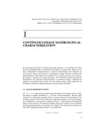
Figure 7.1-4 shows computer printouts of pixels in the upper left corner of a
convolved image for the four types of convolution boundary conditions. In this
example, the source image is constant of maximum value 1.0. The convolution
impulse response array is a uniform array.
7.1.2. Finite-Area Superposition and Convolution: Vector-Space Formulation
If the arrays F and Q of Eq. 7.1-6 are represented in vector form by the vec-
tor f and the vector q, respectively, the finite-area superposition operation
can be written as (2)
(7.1-16)
where D is a matrix containing the elements of the impulse response. It is
convenient to partition the superposition operator matrix D into submatrices of
dimension . Observing the summation limits of Eq. 7.1-7, it is seen that
(7.1-17)
FIGURE 7.1-4 Finite-area convolution boundary conditions, upper left corner of convolved
image.
0.040 0.080 0.120 0.160 0.200 0.200 0.200
0.080 0.160 0.240 0.320 0.400 0.400 0.400
0.120 0.240 0.360 0.480 0.600 0.600 0.600
0.160 0.320 0.480 0.640 0.800 0.800 0.800
0.200 0.400 0.600 0.800 1.000 1.000 1.000
0.200 0.400 0.600 0.800 1.000 1.000 1.000
0.200 0.400 0.600 0.800 1.000 1.000 1.000
0.000 0.000 0.000 0.000 0.000 0.000 0.000
0.000 0.000 0.000 0.000 0.000 0.000 0.000
0.000 0.000 1.000 1.000 1.000 1.000 1.000
0.000 0.000 1.000 1.000 1.000 1.000 1.000
0.000 0.000 1.000 1.000 1.000 1.000 1.000
0.000 0.000 1.000 1.000 1.000 1.000 1.000
0.000 0.000 1.000 1.000 1.000 1.000 1.000

0.360 0.480 0.600 0.600 0.600 0.600 0.600
0.480 0.640 0.800 0.800 0.800 0.800 0.800
0.600 0.800 1.000 1.000 1.000 1.000 1.000
0.600 0.800 1.000 1.000 1.000 1.000 1.000
0.600 0.800 1.000 1.000 1.000 1.000 1.000
0.600 0.800 1.000 1.000 1.000 1.000 1.000
0.600 0.800 1.000 1.000 1.000 1.000 1.000
1.000 1.000 1.000 1.000 1.000 1.000 1.000
1.000 1.000 1.000 1.000 1.000 1.000 1.000
1.000 1.000 1.000 1.000 1.000 1.000 1.000
1.000 1.000 1.000 1.000 1.000 1.000 1.000
1.000 1.000 1.000 1.000 1.000 1.000 1.000
1.000 1.000 1.000 1.000 1.000 1.000 1.000
1.000 1.000 1.000 1.000 1.000 1.000 1.000
(
a
) Upper left corner justified (
b
) Centered, zero boundary
(
c
) Centered, zero padded (
d
) Centered, reflected
55×
N
2
1×
M
2

1×
qDf=
M
2
N
2
×
MN×
D
D
11,
0 …
……
… 0
D
21,
D
22,
0
D
L 1,
D
L 2,
D
ML
–
1 N,
+
0D
L 1

+
1,
0 …
……
… 0D
MN,
=
…
…
…
…
…
…
…
168
SUPERPOSITION AND CONVOLUTION
The general nonzero term of D is then given by
(7.1-18)
Thus, it is observed that D is highly structured and quite sparse, with the center band
of submatrices containing stripes of zero-valued elements.
If the impulse response is position invariant, the structure of D does not depend
explicitly on the output array coordinate . Also,
(7.1-19)
As a result, the columns of D are shifted versions of the first column. Under these
conditions, the finite-area superposition operator is known as the finite-area convo-
lution operator. Figure 7.1-5a contains a notational example of the finite-area con-
volution operator for a (N = 2) input data array, a (M = 4) output data
array, and a (L = 3) impulse response array. The integer pairs (i, j) at each ele-
ment of D represent the element (i, j) of . The basic structure of D can be seen
more clearly in the larger matrix depicted in Figure 7.l-5b. In this example, M = 16,

FIGURE 7.1-5 Finite-area convolution operators: (a) general impulse array, M = 4, N = 2,
L = 3; (b) Gaussian-shaped impulse array, M = 16, N = 8, L = 9.
(
b
)
11
21
31
0
0
11
21
31
0
0
0
0
0
0
0
0
0
0
0
0
0
0
0
0
12

22
32
0
0
12
22
32
11
21
31
0
0
11
21
31
13
23
33
0
0
13
23
33
0
13
23
33
12
22
32

0
0
12
22
32
13
23
33
0
11
21
31
12
22
32
13
23
33
H = D =
(
a
)
D
m
2
n
2
,
m
1

n
1
,()Hm
1
n
1
– 1+ m
2
n
2
1 m
1
m
2
,;+–,()=
m
1
m
2
,()
D
m
2
n
2
,
D
m
2
1

+
n
2
1
+,
=
22× 44×
33×
Hij,()
FINITE-AREA SUPERPOSITION AND CONVOLUTION
169
N = 8, L = 9, and the impulse response has a symmetrical Gaussian shape. Note that
D is a 256 × 64 matrix in this example.
Following the same technique as that leading to Eq. 5.4-7, the matrix form of the
superposition operator may be written as
(7.1-20)
If the impulse response is spatially invariant and is of separable form such that
(7.1-21)
where and are column vectors representing row and column impulse
responses, respectively, then
(7.1-22)
The matrices and are matrices of the form
(7.1-23)
The two-dimensional convolution operation may then be computed by sequential
row and column one-dimensional convolutions. Thus
(7.1-24)
In vector form, the general finite-area superposition or convolution operator requires
operations if the zero-valued multiplications of D are avoided. The separable
operator of Eq. 7.1-24 can be computed with only operations.
QD

mn
,
Fv
n
u
m
T
n 1
=
N
∑
m 1
=
M
∑
=
Hh
C
h
R
T
=
h
R
h
C
DD
C
D
R

⊗=
D
R
D
C
MN×
D
R
h
R
1() 0 … 0
h
R
2() h
R
1()
h
R
3() h
R
2() … 0
h
R
1()
h
R
L()
0
0 … 0 h
R

L()
=
…
…
………
…
QD
C
FD
R
T
=
N
2
L
2
NL M N+()