Tài liệu Xử lý hình ảnh kỹ thuật số P8 pdf

185
8
UNITARY TRANSFORMS
Two-dimensional unitary transforms have found two major applications in image
processing. Transforms have been utilized to extract features from images. For
example, with the Fourier transform, the average value or dc term is proportional to
the average image amplitude, and the high-frequency terms (ac term) give an indica-
tion of the amplitude and orientation of edges within an image. Dimensionality
reduction in computation is a second image processing application. Stated simply,
those transform coefficients that are small may be excluded from processing opera-
tions, such as filtering, without much loss in processing accuracy. Another applica-
tion in the field of image coding is transform image coding, in which a bandwidth
reduction is achieved by discarding or grossly quantizing low-magnitude transform
coefficients. In this chapter we consider the properties of unitary transforms com-
monly used in image processing.
8.1. GENERAL UNITARY TRANSFORMS
A unitary transform is a specific type of linear transformation in which the basic lin-
ear operation of Eq. 5.4-1 is exactly invertible and the operator kernel satisfies cer-
tain orthogonality conditions (1,2). The forward unitary transform of the
image array results in a transformed image array as defined by
(8.1-1)
N
1
N
2
×
Fn
1
n
2
,() N

1
N
2
×
F m
1
m
2
,() Fn
1
n
2
,()An
1
n
2
m
1
m
2
,;,()
n
2
1
=
N
2
∑
n
1

1
=
N
1
∑
=
Digital Image Processing: PIKS Inside, Third Edition. William K. Pratt
Copyright © 2001 John Wiley & Sons, Inc.
ISBNs: 0-471-37407-5 (Hardback); 0-471-22132-5 (Electronic)
186
UNITARY TRANSFORMS
where represents the forward transform kernel. A reverse or
inverse transformation provides a mapping from the transform domain to the image
space as given by
(8.1-2)
where denotes the inverse transform kernel. The transformation is
unitary if the following orthonormality conditions are met:
(8.1-3a)
(8.1-3b)
(8.1-3c)
(8.1-3c)
The transformation is said to be separable if its kernels can be written in the form
(8.1-4a)
(8.1-4b)
where the kernel subscripts indicate row and column one-dimensional transform
operations. A separable two-dimensional unitary transform can be computed in two
steps. First, a one-dimensional transform is taken along each column of the image,
yielding
(8.1-5)
Next, a second one-dimensional unitary transform is taken along each row of

, giving
(8.1-6)
An
1
n
2
m
1
m
2
,;,()
Fn
1
n
2
,() F m
1
m
2
,()Bn
1
n
2
m
1
m
2
,;,()
m
2

1
=
N
2
∑
m
1
1
=
N
1
∑
=
Bn
1
n
2
m
1
m
2
,;,()
An
1
n
2
m
1
m
2

,;,()A
∗
j
1
j
2
m
1
m
2
,;,()
m
2
∑
m
1
∑
δ n
1
j
1
– n
2
j
2
–,()=
Bn
1
n
2

m
1
m
2
,;,()B
∗
j
1
j
2
m
1
m
2
,;,()
m
2
∑
m
1
∑
δ n
1
j
1
– n
2
j
2
–,()=

An
1
n
2
m
1
m
2
,;,()A
∗
n
1
n
2
k
1
k
2
,;,()
n
2
∑
n
1
∑
δ m
1
k
1
– m

2
k
2
–,()=
Bn
1
n
2
m
1
m
2
,;,()B
∗
n
1
n
2
k
1
k
2
,;,()
n
2
∑
n
1
∑
δ m

1
k
1
– m
2
k
2
–,()=
An
1
n
2
m
1
m
2
,;,()A
C
n
1
m
1
,()A
R
n
2
m
2
,()=
Bn

1
n
2
m
1
m
2
,;,()B
C
n
1
m
1
,()B
R
n
2
m
2
,()=
Pm
1
n
2
,() Fn
1
n
2
,()A
C

n
1
m
1
,()
n
1
1
=
N
1
∑
=
Pm
1
n
2
,()
F m
1
m
2
,() Pm
1
n
2
,()A
R
n
2

m
2
,()
n
2
1
=
N
2
∑
=
GENERAL UNITARY TRANSFORMS
187
Unitary transforms can conveniently be expressed in vector-space form (3). Let F
and f denote the matrix and vector representations of an image array, and let and
be the matrix and vector forms of the transformed image. Then, the two-dimen-
sional unitary transform written in vector form is given by
(8.1-7)
where A is the forward transformation matrix. The reverse transform is
(8.1-8)
where B represents the inverse transformation matrix. It is obvious then that
(8.1-9)
For a unitary transformation, the matrix inverse is given by
(8.1-10)
and A is said to be a unitary matrix. A real unitary matrix is called an orthogonal
matrix. For such a matrix,
(8.1-11)
If the transform kernels are separable such that
(8.1-12)
where and are row and column unitary transform matrices, then the trans-

formed image matrix can be obtained from the image matrix by
(8.1-13a)
The inverse transformation is given by
(8.1-13b)
F
f
ff
f
f
ff
f Af=
fBf
ff
f=
BA
1
–
=
A
1
–
A
∗
T
=
A
1
–
A
T

=
AA
C
A
R
⊗=
A
R
A
C
F A
C
FA
R
T
=
F B
C
F B
R
T
=
188
UNITARY TRANSFORMS
where and .
Separable unitary transforms can also be expressed in a hybrid series–vector
space form as a sum of vector outer products. Let and represent rows
n
1
and n

2
of the unitary matrices A
R
and A
R
, respectively. Then, it is easily verified
that
(8.1-14a)
Similarly,
(8.1-14b)
where and denote rows m
1
and m
2
of the unitary matrices B
C
and
B
R
, respectively. The vector outer products of Eq. 8.1-14 form a series of matrices,
called basis matrices, that provide matrix decompositions of the image matrix F or
its unitary transformation F.
There are several ways in which a unitary transformation may be viewed. An
image transformation can be interpreted as a decomposition of the image data into a
generalized two-dimensional spectrum (4). Each spectral component in the trans-
form domain corresponds to the amount of energy of the spectral function within the
original image. In this context, the concept of frequency may now be generalized to
include transformations by functions other than sine and cosine waveforms. This
type of generalized spectral analysis is useful in the investigation of specific decom-
positions that are best suited for particular classes of images. Another way to visual-

ize an image transformation is to consider the transformation as a multidimensional
rotation of coordinates. One of the major properties of a unitary transformation is
that measure is preserved. For example, the mean-square difference between two
images is equal to the mean-square difference between the unitary transforms of the
images. A third approach to the visualization of image transformation is to consider
Eq. 8.1-2 as a means of synthesizing an image with a set of two-dimensional mathe-
matical functions for a fixed transform domain coordinate
. In this interpretation, the kernel is called a two-dimen-
sional basis function and the transform coefficient is the amplitude of the
basis function required in the synthesis of the image.
In the remainder of this chapter, to simplify the analysis of two-dimensional uni-
tary transforms, all image arrays are considered square of dimension N. Further-
more, when expressing transformation operations in series form, as in Eqs. 8.1-1
and 8.1-2, the indices are renumbered and renamed. Thus the input image array is
denoted by F(j, k) for j, k = 0, 1, 2,..., N - 1, and the transformed image array is rep-
resented by F(u, v) for u, v = 0, 1, 2,..., N - 1. With these definitions, the forward uni-
tary transform becomes
B
C
A
C
1
–
=B
R
A
R
1
–
=

a
C
n
1
() a
R
n
2
()
F Fn
1
n
2
,()a
C
n
1
()a
R
T
n
2
()
n
2
1
=
N
2
∑

n
1
1
=
N
1
∑
=
F F m
1
m
2
,()b
C
m
1
()b
R
T
m
2
()
m
2
1
=
N
2
∑
m

1
1
=
N
1
∑
=
b
C
m
1
() b
R
m
2
()
Bn
1
n
2
m
1
m
2
,;,()
m
1
m
2
,() Bn

1
n
2
m
1
m
2
,;,()
F m
1
m
2
,()
FOURIER TRANSFORM
189
(8.1-15a)
and the inverse transform is
(8.1-15b)
8.2. FOURIER TRANSFORM
The discrete two-dimensional Fourier transform of an image array is defined in
series form as (5–10)
(8.2-1a)
where , and the discrete inverse transform is given by
(8.2-1b)
The indices (u, v) are called the spatial frequencies of the transformation in analogy
with the continuous Fourier transform. It should be noted that Eq. 8.2-1 is not uni-
versally accepted by all authors; some prefer to place all scaling constants in the
inverse transform equation, while still others employ a reversal in the sign of the
kernels.
Because the transform kernels are separable and symmetric, the two dimensional

transforms can be computed as sequential row and column one-dimensional trans-
forms. The basis functions of the transform are complex exponentials that may be
decomposed into sine and cosine components. The resulting Fourier transform pairs
then become
(8.2-2a)
(8.2-2b)
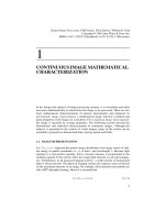
Figure 8.2-1 shows plots of the sine and cosine components of the one-dimensional
Fourier basis functions for N = 16. It should be observed that the basis functions are
a rough approximation to continuous sinusoids only for low frequencies; in fact, the
F uv,() Fjk,()Ajkuv,;,()
k 0
=
N 1
–
∑
j 0
=
N 1
–
∑
=
Fjk,() F uv,()Bjkuv,;,()
v 0
=
N 1
–
∑
u 0
=
N 1

–
∑
=
F uv,()
1
N
---- Fjk,()
2πi–
N
----------- uj vk+()



exp
k 0
=
N 1
–
∑
j 0
=
N 1
–
∑
=
i 1–=
Fjk,()
1
N
---- F uv,()

2πi
N
-------- uj vk+()



exp
v 0
=
N 1
–
∑
u 0
=
N 1
–
∑
=
Ajk uv,;,()
2πi–
N
----------- uj vk+()



exp
2π
N
------ uj vk+()




cos i
2π
N
------ uj vk+()



sin–==
Bjkuv,;,()
2πi
N
-------- uj vk+()



exp
2π
N
------ uj vk+()



cos i
2π
N
------ uj vk+()




sin+==
190
UNITARY TRANSFORMS
highest-frequency basis function is a square wave. Also, there are obvious redun-
dancies between the sine and cosine components.
The Fourier transform plane possesses many interesting structural properties.
The spectral component at the origin of the Fourier domain
(8.2-3)
is equal to N times the spatial average of the image plane. Making the substitutions
, in Eq. 8.2-1, where m and n are constants, results in
FIGURE 8.2-1 Fourier transform basis functions, N = 16.
F 00,()
1
N
---- Fjk,()
k 0
=
N 1
–
∑
j 0
=
N 1
–
∑
=
uumN+= vvnN+=
FOURIER TRANSFORM
191

(8.2-4)
For all integer values of m and n, the second exponential term of Eq. 8.2-5 assumes
a value of unity, and the transform domain is found to be periodic. Thus, as shown in
Figure 8.2-2a,
(8.2-5)
for .
The two-dimensional Fourier transform of an image is essentially a Fourier series
representation of a two-dimensional field. For the Fourier series representation to be
valid, the field must be periodic. Thus, as shown in Figure 8.2-2b, the original image
must be considered to be periodic horizontally and vertically. The right side of the
image therefore abuts the left side, and the top and bottom of the image are adjacent.
Spatial frequencies along the coordinate axes of the transform plane arise from these
transitions.
If the image array represents a luminance field, will be a real positive
function. However, its Fourier transform will, in general, be complex. Because the
transform domain contains

components, the real and imaginary, or phase and
magnitude components, of each coefficient, it might be thought that the Fourier
transformation causes an increase in dimensionality. This, however, is not the case
because exhibits a property of conjugate symmetry. From Eq. 8.2-4, with m
and n set to integer values, conjugation yields
FIGURE 8.2-2. Periodic image and Fourier transform arrays.
F umN+ vnN+,()
1
N
---- Fjk,()
2πi–
N
----------- uj vk+()




exp 2πi– mj nk+(){}exp
k 0
=
N 1
–
∑
j 0
=
N 1
–
∑
=
F umN+ vnN+,()F uv,()=
mn, 012…,±,±,=
Fjk,()
2N
2
F uv,()
192
UNITARY TRANSFORMS
(8.2-6)
By the substitution and it can be shown that
(8.2-7)
for . As a result of the conjugate symmetry property, almost one-
half of the transform domain samples are redundant; that is, they can be generated
from other transform samples. Figure 8.2-3 shows the transform plane with a set of
redundant components crosshatched. It is possible, of course, to choose the left half-

plane samples rather than the upper plane samples as the nonredundant set.
Figure 8.2-4 shows a monochrome test image and various versions of its Fourier
transform, as computed by Eq. 8.2-1a, where the test image has been scaled over
unit range . Because the dynamic range of transform components is
much larger than the exposure range of photographic film, it is necessary to com-
press the coefficient values to produce a useful display. Amplitude compression to a
unit range display array can be obtained by clipping large-magnitude values
according to the relation
FIGURE 8.2-3. Fourier transform frequency domain.
F * umN+ vnN+,()
1
N
---- Fjk,()
2πi–
N
----------- uj vk+()



exp
k 0
=
N 1
–
∑
j 0
=
N 1
–
∑

=
uu–= vv–=
F uv,()F
*
u– mN+ v– nN+,()=
n 012…,±,±,=
0.0 Fjk,()1.0≤≤
D uv,()
FOURIER TRANSFORM
193
if (8.2-8a)
if (8.2-8b)
where is the clipping factor and is the maximum coefficient
magnitude. Another form of amplitude compression is to take the logarithm of each
component as given by
(8.2-9)
FIGURE 8.2-4. Fourier transform of the smpte_girl_luma image.
(
a
) Original (
b
) Clipped magnitude, nonordered
(
c
) Log magnitude, nonordered (
d
) Log magnitude, ordered
D uv,()
1.0
F uv,()

c F
max
---------------------





=
F uv,()c F
max
≥
F uv,()c F
max
<
0.0 c< 1.0≤ F
max
D uv,()
abF uv,()+{}log
abF
max
+{}log
-------------------------------------------------=
194
UNITARY TRANSFORMS
where a and b are scaling constants. Figure 8.2-4b is a clipped magnitude display of
the magnitude of the Fourier transform coefficients. Figure 8.2-4c is a logarithmic
display for a = 1.0 and b = 100.0.
In mathematical operations with continuous signals, the origin of the transform
domain is usually at its geometric center. Similarly, the Fraunhofer diffraction pat-

tern of a photographic transparency of transmittance produced by a coher-
ent optical system has its zero-frequency term at the center of its display. A
computer-generated two-dimensional discrete Fourier transform with its origin at its
center can be produced by a simple reordering of its transform coefficients. Alterna-
tively, the quadrants of the Fourier transform, as computed by Eq. 8.2-la, can be
reordered automatically by multiplying the image function by the factor
prior to the Fourier transformation. The proof of this assertion follows from Eq.
8.2-4 with the substitution . Then, by the identity
(8.2-10)
Eq. 8.2-5 can be expressed as
(8.2-11)
Figure 8.2-4d contains a log magnitude display of the reordered Fourier compo-
nents. The conjugate symmetry in the Fourier domain is readily apparent from the
photograph.
The Fourier transform written in series form in Eq. 8.2-1 may be redefined in
vector-space form as
(8.2-12a)
(8.2-12b)
where f and are vectors obtained by column scanning the matrices F and F,
respectively. The transformation matrix A can be written in direct product form as
(8.2-13)
Fxy,()
1–()
jk
+
mn
1
2
---
==

iπ jk+(){}exp 1–()
jk
+
=
F uN2⁄+ vN2⁄+,()
1
N
---- Fjk,()1–()
jk
+
2πi–
N
----------- uj vk+()



exp
k 0
=
N 1
–
∑
j 0
=
N 1
–
∑
=
f
ff

f Af=
fA
∗
T
f
ff
f=
f
ff
f
AA
C
A
R
⊗=
COSINE, SINE, AND HARTLEY TRANSFORMS
195
where
(8.2-14)
with . As a result of the direct product decomposition of A, the
image matrix and transformed image matrix are related by
(8.2-15a)
(8.2-15b)
The properties of the Fourier transform previously proved in series form obviously
hold in the matrix formulation.
One of the major contributions to the field of image processing was the discovery
(5) of an efficient computational algorithm for the discrete Fourier transform (DFT).
Brute-force computation of the discrete Fourier transform of a one-dimensional
sequence of N values requires on the order of complex multiply and add opera-
tions. A fast Fourier transform (FFT) requires on the order of operations.

For large images the computational savings are substantial. The original FFT algo-
rithms were limited to images whose dimensions are a power of 2 (e.g.,
). Modern algorithms exist for less restrictive image dimensions.
Although the Fourier transform possesses many desirable analytic properties, it
has a major drawback: Complex, rather than real number computations are
necessary. Also, for image coding it does not provide as efficient image energy
compaction as other transforms.
8.3. COSINE, SINE, AND HARTLEY TRANSFORMS
The cosine, sine, and Hartley transforms are unitary transforms that utilize
sinusoidal basis functions, as does the Fourier transform. The cosine and sine
transforms are not simply the cosine and sine parts of the Fourier transform. In fact,
the cosine and sine parts of the Fourier transform, individually, are not orthogonal
functions. The Hartley transform jointly utilizes sine and cosine basis functions, but
its coefficients are real numbers, as contrasted with the Fourier transform whose
coefficients are, in general, complex numbers.
A
R
A
C
W
0
W
0
W
0
… W
0
W
0
W

1
W
2
… W
N 1
–
W
0
W
2
W
4
… W
2 N 1
–
()
W
0
··
… W
N 1
–
()
2
==
…
…
W 2πi– N⁄{
}
exp=

F A
C
FA
R
=
F A
C
∗
F A
R
∗
=
N
2
NNlog
N 2
9
512==