Tài liệu Minimization or Maximization of Functions part 9 pdf
Bạn đang xem bản rút gọn của tài liệu. Xem và tải ngay bản đầy đủ của tài liệu tại đây (232.62 KB, 15 trang )
430
Chapter 10. Minimization or Maximization of Functions
Sample page from NUMERICAL RECIPES IN C: THE ART OF SCIENTIFIC COMPUTING (ISBN 0-521-43108-5)
Copyright (C) 1988-1992 by Cambridge University Press.Programs Copyright (C) 1988-1992 by Numerical Recipes Software.
Permission is granted for internet users to make one paper copy for their own personal use. Further reproduction, or any copying of machine-
readable files (including this one) to any servercomputer, is strictly prohibited. To order Numerical Recipes books,diskettes, or CDROMs
visit website or call 1-800-872-7423 (North America only),or send email to (outside North America).
Quasi-Newton methods like dfpmin work well with the approximate line
minimization done by lnsrch. The routines powell (§10.5) and frprmn (§10.6),
however, need more accurate line minimization, which is carried out by the routine
linmin.
Advanced Implementations of Variable Metric Methods
Although rare, it can conceivably happen that roundoff errors cause the matrix H
i
to
become nearly singular or non-positive-definite. This can be serious, because the supposed
search directions might then not lead downhill, and because nearly singular H
i
’s tend to give
subsequent H
i
’s that are also nearly singular.
There is a simple fix for this rare problem, the same as was mentioned in §10.4: In case
of any doubt, you should restart the algorithm at the claimed minimum point, and see if it
goes anywhere. Simple, but not very elegant. Modern implementations of variable metric
methods deal with the problem in a more sophisticated way.
Instead ofbuildingupanapproximationtoA
−1
, itispossible tobuild up anapproximation
of A itself. Then, instead of calculating the left-hand side of (10.7.4) directly, one solves
the set of linear equations
A · (x
m
− x
i
)=−∇f(x
i
)(10.7.11)
At first glance this seems like a bad idea, since solving (10.7.11) is a process of order
N
3
— and anyway, how does this help the roundoff problem? The trick is not to store A but
rather a triangular decomposition of A, its Cholesky decomposition (cf. §2.9). The updating
formula used for the Cholesky decomposition of A is of order N
2
and can be arranged to
guarantee that the matrix remains positive definite and nonsingular, even in the presence of
finite roundoff. This method is due to Gill and Murray
[1,2]
.
CITED REFERENCES AND FURTHER READING:
Dennis, J.E., and Schnabel, R.B. 1983,
Numerical Methods for Unconstrained Optimization and
Nonlinear Equations
(Englewood Cliffs, NJ: Prentice-Hall). [1]
Jacobs, D.A.H. (ed.) 1977,
The State of the Art in Numerical Analysis
(London: Academic Press),
Chapter III.1,
§§
3–6 (by K. W. Brodlie). [2]
Polak, E. 1971,
Computational Methods in Optimization
(New York: Academic Press), pp. 56ff. [3]
Acton, F.S. 1970,
Numerical Methods That Work
; 1990, corrected edition (Washington: Mathe-
matical Association of America), pp. 467–468.
10.8 Linear Programming and the Simplex
Method
The subject of linear programming, sometimes called linear optimization,
concerns itselfwiththe followingproblem: For N independentvariables x
1
,...,x
N
,
maximize the function
z = a
01
x
1
+ a
02
x
2
+ ···+a
0N
x
N
(10.8.1)
subject to the primary constraints
x
1
≥ 0,x
2
≥0, ... x
N
≥0(10.8.2)
10.8 Linear Programming and the Simplex Method
431
Sample page from NUMERICAL RECIPES IN C: THE ART OF SCIENTIFIC COMPUTING (ISBN 0-521-43108-5)
Copyright (C) 1988-1992 by Cambridge University Press.Programs Copyright (C) 1988-1992 by Numerical Recipes Software.
Permission is granted for internet users to make one paper copy for their own personal use. Further reproduction, or any copying of machine-
readable files (including this one) to any servercomputer, is strictly prohibited. To order Numerical Recipes books,diskettes, or CDROMs
visit website or call 1-800-872-7423 (North America only),or send email to (outside North America).
and simultaneously subject to M = m
1
+ m
2
+ m
3
additional constraints, m
1
of
them of the form
a
i1
x
1
+ a
i2
x
2
+ ···+a
iN
x
N
≤ b
i
(b
i
≥ 0) i =1,...,m
1
(10.8.3)
m
2
of them of the form
a
j1
x
1
+ a
j2
x
2
+ ···+a
jN
x
N
≥ b
j
≥ 0 j = m
1
+1,...,m
1
+m
2
(10.8.4)
and m
3
of them of the form
a
k1
x
1
+ a
k2
x
2
+ ···+a
kN
x
N
= b
k
≥ 0
k = m
1
+ m
2
+1,...,m
1
+m
2
+m
3
(10.8.5)
The various a
ij
’s can have either sign, or be zero. The fact that the b’s must all be
nonnegative (as indicated by the final inequality in the above three equations) is a
matter of convention only, since you can multiply any contrary inequality by −1.
There is no particular significance in the number of constraints M being less than,
equal to, or greater than the number of unknowns N.
A set of values x
1
...x
N
that satisfies the constraints (10.8.2)–(10.8.5) is called
a feasible vector. The function that we are trying to maximize is called the objective
function. The feasible vector that maximizes the objective function is called the
optimal feasible vector. An optimal feasible vector can fail to exist for two distinct
reasons: (i) there are no feasible vectors, i.e., the given constraints are incompatible,
or (ii) there is no maximum, i.e., there is a direction in N space where one or more
of the variables can be taken to infinity while still satisfying the constraints, giving
an unbounded value for the objective function.
As you see, the subject of linear programming is surrounded by notational and
terminological thickets. Both of these thorny defenses are lovingly cultivated by a
coterie of stern acolytes who have devoted themselves to the field. Actually, the
basic ideas of linear programming are quite simple. Avoiding the shrubbery, we
want to teach you the basics by means of a couple of specific examples; it should
then be quite obvious how to generalize.
Why is linear programming so important? (i) Because “nonnegativity” is the
usual constraint on any variable x
i
that represents the tangible amount of some
physical commodity, like guns, butter, dollars, units of vitamin E, food calories,
kilowatt hours, mass, etc. Hence equation (10.8.2). (ii) Because one is often
interested in additive (linear) limitations or bounds imposed by man or nature:
minimum nutritionalrequirement, maximum affordable cost, maximum on available
labor or capital, minimum tolerable level of voter approval, etc. Hence equations
(10.8.3)–(10.8.5). (iii) Because the function that one wants to optimize may be
linear, or else may at least be approximated by a linear function — since that is the
problem that linear programming can solve. Hence equation (10.8.1). For a short,
semipopular survey of linear programming applications, see Bland
[1]
.
Here is a specific example of a problem in linear programming, which has
N =4,m
1
=2,m
2
=m
3
=1, hence M =4:
Maximize z = x
1
+ x
2
+3x
3
−
1
2
x
4
(10.8.6)
432
Chapter 10. Minimization or Maximization of Functions
Sample page from NUMERICAL RECIPES IN C: THE ART OF SCIENTIFIC COMPUTING (ISBN 0-521-43108-5)
Copyright (C) 1988-1992 by Cambridge University Press.Programs Copyright (C) 1988-1992 by Numerical Recipes Software.
Permission is granted for internet users to make one paper copy for their own personal use. Further reproduction, or any copying of machine-
readable files (including this one) to any servercomputer, is strictly prohibited. To order Numerical Recipes books,diskettes, or CDROMs
visit website or call 1-800-872-7423 (North America only),or send email to (outside North America).
additional constraint (inequality)
additional constraint (inequality)
the optimal feasible vector
some feasible vectors
x
1
primary constraint
x
2
a feasible basic vector
(not optimal)
primary constraint
additional constraint (equality)
z
=
3.1
z
=
2.9
z
=
2.8
z
=
2.7
z
=
2.6
z
=
2.5
z
=
2.4
z
=
3.0
Figure 10.8.1. Basic concepts of linear programming. The case of only two independent variables,
x
1
,x
2
, is shown. The linear function z, to be maximized, is represented by its contour lines. Primary
constraints require x
1
and x
2
to be positive. Additional constraints may restrict the solution to regions
(inequality constraints) or to surfaces of lower dimensionality (equality constraints). Feasible vectors
satisfy all constraints. Feasible basic vectors also lie on the boundary of the allowed region. The simplex
method steps among feasible basic vectors until the optimal feasible vector is found.
with all the x’s nonnegative and also with
x
1
+2x
3
≤740
2x
2
− 7x
4
≤ 0
x
2
− x
3
+2x
4
≥
1
2
x
1
+x
2
+x
3
+x
4
=9
(10.8.7)
The answer turns out to be (to 2 decimals) x
1
=0,x
2
=3.33, x
3
=4.73, x
4
=0.95.
In the rest of this section we will learn how this answer is obtained. Figure 10.8.1
summarizes some of the terminology thus far.
Fundamental Theorem of Linear Optimization
Imagine that westart with afull N-dimensionalspaceof candidatevectors. Then
(in mind’s eye, at least) we carve away the regions that are eliminated in turn by each
imposed constraint. Since the constraints are linear, every boundary introduced by
this process is a plane, or rather hyperplane. Equality constraints of the form (10.8.5)
10.8 Linear Programming and the Simplex Method
433
Sample page from NUMERICAL RECIPES IN C: THE ART OF SCIENTIFIC COMPUTING (ISBN 0-521-43108-5)
Copyright (C) 1988-1992 by Cambridge University Press.Programs Copyright (C) 1988-1992 by Numerical Recipes Software.
Permission is granted for internet users to make one paper copy for their own personal use. Further reproduction, or any copying of machine-
readable files (including this one) to any servercomputer, is strictly prohibited. To order Numerical Recipes books,diskettes, or CDROMs
visit website or call 1-800-872-7423 (North America only),or send email to (outside North America).
force the feasible region onto hyperplanes of smaller dimension, while inequalities
simply divide the then-feasible region into allowed and nonallowed pieces.
When all the constraints are imposed, either we are left with some feasible
region or else there are no feasible vectors. Since the feasible region is bounded by
hyperplanes, it is geometrically a kind of convex polyhedron or simplex (cf. §10.4).
If there is a feasible region, can the optimal feasible vector be somewhere in its
interior, away from the boundaries? No, because the objective function is linear.
This means that it always has a nonzero vector gradient. This, in turn, means that
we could always increase the objective function by running up the gradient until
we hit a boundary wall.
The boundaryof any geometrical region has one less dimension than its interior.
Therefore, we can now run up the gradient projected into the boundary wall until we
reach an edge of that wall. We can then run up that edge, and so on, down through
whatever number of dimensions, until we finally arrive at a point, a vertex of the
original simplex. Since this point has all N of its coordinates defined, it must be
the solution of N simultaneous equalities drawn from the original set of equalities
and inequalities (10.8.2)–(10.8.5).
Points that are feasible vectors and that satisfy N of the original constraints
as equalities, are termed feasible basic vectors.IfN>M, then a feasible basic
vector has at least N − M of its components equal to zero, since at least that many
of the constraints (10.8.2) will be needed to make up the total of N. Put the other
way, at most M components of a feasible basic vector are nonzero. In the example
(10.8.6)–(10.8.7), you can check that the solution as given satisfies as equalities the
last three constraints of (10.8.7) and the constraint x
1
≥ 0, for the required total of 4.
Put together the two preceding paragraphs and you have the Fundamental
Theorem of Linear Optimization: If an optimal feasible vector exists, then there is a
feasible basic vector that is optimal. (Didn’t we warn you about the terminological
thicket?)
The importance of the fundamental theorem is that it reduces the optimization
problem to a “combinatorial” problem, that of determining which N constraints
(out of the M + N constraints in 10.8.2–10.8.5) should be satisfied by the optimal
feasible vector. We have only to keep trying different combinations, and computing
the objective function for each trial, until we find the best.
Doing this blindly would take halfway to forever. The simplex method,first
published by Dantzig in 1948 (see
[2]
), is a way of organizing the procedure so that
(i) a series of combinations is tried for which the objective function increases at each
step, and (ii) the optimal feasible vector is reached after a number of iterations that
is almost always no larger than of order M or N, whichever is larger. An interesting
mathematical sidelight is that this second property, although known empirically ever
since the simplex method was devised, was not proved to be true until the 1982 work
of Stephen Smale. (For a contemporary account, see
[3]
.)
Simplex Method for a Restricted Normal Form
A linear programming problem is said to be in normal form if it has no
constraints in the form (10.8.3) or (10.8.4), but rather only equality constraints of the
form (10.8.5) and nonnegativity constraints of the form (10.8.2).
434
Chapter 10. Minimization or Maximization of Functions
Sample page from NUMERICAL RECIPES IN C: THE ART OF SCIENTIFIC COMPUTING (ISBN 0-521-43108-5)
Copyright (C) 1988-1992 by Cambridge University Press.Programs Copyright (C) 1988-1992 by Numerical Recipes Software.
Permission is granted for internet users to make one paper copy for their own personal use. Further reproduction, or any copying of machine-
readable files (including this one) to any servercomputer, is strictly prohibited. To order Numerical Recipes books,diskettes, or CDROMs
visit website or call 1-800-872-7423 (North America only),or send email to (outside North America).
For our purposes it will be useful to consider an even more restricted set of
cases, with this additional property: Each equality constraint of the form (10.8.5)
must have at least one variable that has a positive coefficient and that appears
uniquely in that one constraint only. We can then choose one such variable in each
constraint equation, and solve that constraint equation for it. The variables thus
chosen are called left-hand variables or basic variables, and there are exactly M
(= m
3
) of them. The remaining N − M variables are called right-hand variables or
nonbasic variables. Obviously this restricted normal form can be achieved only in
the case M ≤ N, so that is the case that we will consider.
You may be thinking that our restricted normal form is so specialized that
it is unlikely to include the linear programming problem that you wish to solve.
Not at all! We will presently show how any linear programming problem can be
transformed into restricted normal form. Therefore bear with us and learn how to
apply the simplex method to a restricted normal form.
Here is an example of a problem in restricted normal form:
Maximize z =2x
2
−4x
3
(10.8.8)
with x
1
, x
2
, x
3
,andx
4
all nonnegative and also with
x
1
=2−6x
2
+x
3
x
4
=8+3x
2
−4x
3
(10.8.9)
This example has N =4,M=2; the left-hand variables are x
1
and x
4
;the
right-hand variables are x
2
and x
3
. The objective function (10.8.8) is written so
as to depend only on right-hand variables; note, however, that this is not an actual
restriction on objective functions in restricted normal form, since any left-hand
variables appearing in the objective function could be eliminated algebraically by
use of (10.8.9) or its analogs.
For any problem in restricted normal form, we can instantly read off a feasible
basic vector (although not necessarily the optimal feasible basic vector). Simply set
all right-hand variables equal to zero, and equation (10.8.9) then gives the values of
the left-hand variables for which the constraintsare satisfied. The idea of the simplex
method is to proceed by a series of exchanges. In each exchange, a right-hand
variable and a left-hand variable change places. At each stage we maintain a problem
in restricted normal form that is equivalent to the original problem.
It is notationally convenient to record the information content of equations
(10.8.8) and (10.8.9) in a so-called tableau, as follows:
x
2
x
3
z 0 2 −4
x
1
2 −6 1
x
4
8 3 −4
(10.8.10)
You should study (10.8.10) to be sure that you understand where each entry comes
from, and how to translate back and forth between the tableau and equation formats
of a problem in restricted normal form.
10.8 Linear Programming and the Simplex Method
435
Sample page from NUMERICAL RECIPES IN C: THE ART OF SCIENTIFIC COMPUTING (ISBN 0-521-43108-5)
Copyright (C) 1988-1992 by Cambridge University Press.Programs Copyright (C) 1988-1992 by Numerical Recipes Software.
Permission is granted for internet users to make one paper copy for their own personal use. Further reproduction, or any copying of machine-
readable files (including this one) to any servercomputer, is strictly prohibited. To order Numerical Recipes books,diskettes, or CDROMs
visit website or call 1-800-872-7423 (North America only),or send email to (outside North America).
The first step in the simplex method is to examine the top row of the tableau,
which we will call the “z-row.” Look at the entries in columns labeled by right-hand
variables (we will call these “right-columns”). We want to imagine in turn the effect
of increasing each right-hand variable from its present value of zero, while leaving
all the other right-hand variables at zero. Will the objective function increase or
decrease? The answer is given by the sign of the entry in the z-row. Since we want
to increase the objective function, only right columns having positive z-row entries
are of interest. In (10.8.10) there is only one such column, whose z-row entry is 2.
The second step is to examine the column entries below each z-row entry
that was selected by step one. We want to ask how much we can increase the
right-hand variable before one of the left-hand variables is driven negative, which is
not allowed. If the tableau element at the intersection of the right-hand column and
the left-hand variable’s row is positive, thenit poses no restriction: the corresponding
left-hand variable will just be driven more and more positive. If all the entries in
any right-hand column are positive, then there is no bound on the objective function
and (having said so) we are done with the problem.
If one or more entries below a positive z-row entry are negative, then we have
to figure out which such entry first limits the increase of that column’s right-hand
variable. Evidently the limitingincrease is given by dividingthe element in the right-
hand column (which is called the pivot element) into the element in the “constant
column” (leftmost column) of the pivot element’s row. A value that is small in
magnitude is most restrictive. The increase in the objective function for this choice
of pivot element is then that value multiplied by the z-row entry of that column. We
repeat this procedure on all possible right-hand columns to find the pivot element
with the largest such increase. That completes our “choice of a pivot element.”
In the above example, the only positive z-row entry is 2. There is only one
negative entry below it, namely −6, so this is the pivot element. Its constant-column
entry is 2. This pivot will therefore allow x
2
to be increased by 2 ÷|6|, which results
in an increase of the objective function by an amount (2 × 2) ÷|6|.
The third step is to do the increase of the selected right-hand variable, thus
making it a left-hand variable; and simultaneously to modify the left-hand variables,
reducing the pivot-row element to zero and thus making it a right-hand variable. For
our above example let’s do this first by hand: We begin by solving the pivot-row
equation for the new left-hand variable x
2
in favor of the old one x
1
, namely
x
1
=2−6x
2
+x
3
→ x
2
=
1
3
−
1
6
x
1
+
1
6
x
3
(10.8.11)
We then substitute this into the old z-row,
z =2x
2
−4x
3
=2
1
3
−
1
6
x
1
+
1
6
x
3
−4x
3
=
2
3
−
1
3
x
1
−
11
3
x
3
(10.8.12)
and into all other left-variable rows, in this case only x
4
,
x
4
=8+3
1
3
−
1
6
x
1
+
1
6
x
3
−4x
3
=9−
1
2
x
1
−
7
2
x
3
(10.8.13)