Tài liệu Integration of Ordinary Differential Equations part 3 doc

714
Chapter 16. Integration of Ordinary Differential Equations
Sample page from NUMERICAL RECIPES IN C: THE ART OF SCIENTIFIC COMPUTING (ISBN 0-521-43108-5)
Copyright (C) 1988-1992 by Cambridge University Press.Programs Copyright (C) 1988-1992 by Numerical Recipes Software.
Permission is granted for internet users to make one paper copy for their own personal use. Further reproduction, or any copying of machine-
readable files (including this one) to any servercomputer, is strictly prohibited. To order Numerical Recipes books,diskettes, or CDROMs
visit website or call 1-800-872-7423 (North America only),or send email to (outside North America).
dv=vector(1,nvar);
for (i=1;i<=nvar;i++) { Load starting values.
v[i]=vstart[i];
y[i][1]=v[i];
}
xx[1]=x1;
x=x1;
h=(x2-x1)/nstep;
for (k=1;k<=nstep;k++) { Take nstep steps.
(*derivs)(x,v,dv);
rk4(v,dv,nvar,x,h,vout,derivs);
if ((float)(x+h) == x) nrerror("Step size too small in routine rkdumb");
x+=h;
xx[k+1]=x; Store intermediate steps.
for (i=1;i<=nvar;i++) {
v[i]=vout[i];
y[i][k+1]=v[i];
}
}
free_vector(dv,1,nvar);
free_vector(vout,1,nvar);
free_vector(v,1,nvar);
}
CITED REFERENCES AND FURTHER READING:

Abramowitz, M., and Stegun, I.A. 1964,
Handbook of Mathematical Functions
, Applied Mathe-
matics Series, Volume 55 (Washington: National Bureau of Standards; reprinted 1968 by
Dover Publications, New York),
§
25.5. [1]
Gear, C.W. 1971,
Numerical Initial Value Problems in Ordinary Differential Equations
(Englewood
Cliffs, NJ: Prentice-Hall), Chapter 2. [2]
Shampine, L.F., and Watts, H.A. 1977, in
Mathematical Software III
, J.R. Rice, ed. (New York:
Academic Press), pp. 257–275; 1979,
Applied Mathematics and Computation
,vol.5,
pp. 93–121. [3]
Rice, J.R. 1983,
Numerical Methods, Software, and Analysis
(New York: McGraw-Hill),
§
9.2.
16.2 Adaptive Stepsize Control for Runge-Kutta
AgoodODEintegratorshouldexertsomeadaptivecontroloveritsownprogress,
making frequent changes in its stepsize. Usually the purposeof this adaptive stepsize
control is to achieve some predetermined accuracy in the solution with minimum
computational effort. Many small steps should tiptoe through treacherous terrain,
while a few great strides should speed through smooth uninteresting countryside.
The resulting gains in efficiency are not mere tens of percents or factors of two;

they can sometimes be factors of ten, a hundred, or more. Sometimes accuracy
may be demanded not directly in the solution itself, but in some related conserved
quantity that can be monitored.
Implementationof adaptive stepsize controlrequires that the steppingalgorithm
signal information about itsperformance,most important,anestimate ofitstruncation
error. In this section we willlearn how such informationcan beobtained. Obviously,
16.2 Adaptive Stepsize Control for Runge-Kutta
715
Sample page from NUMERICAL RECIPES IN C: THE ART OF SCIENTIFIC COMPUTING (ISBN 0-521-43108-5)
Copyright (C) 1988-1992 by Cambridge University Press.Programs Copyright (C) 1988-1992 by Numerical Recipes Software.
Permission is granted for internet users to make one paper copy for their own personal use. Further reproduction, or any copying of machine-
readable files (including this one) to any servercomputer, is strictly prohibited. To order Numerical Recipes books,diskettes, or CDROMs
visit website or call 1-800-872-7423 (North America only),or send email to (outside North America).
the calculation of this information will add to the computational overhead, but the
investment will generally be repaid handsomely.
With fourth-order Runge-Kutta, the most straightforward technique by far is
step doubling (see, e.g.,
[1]
). We take each step twice, once as a full step, then,
independently, as two half steps (see Figure 16.2.1). How much overhead is this,
say in terms of the number of evaluations of the right-hand sides? Each of the
three separate Runge-Kutta steps in the procedure requires 4 evaluations, but the
single and double sequences share a starting point, so the total is 11. This is to be
compared not to 4, but to 8 (the two half-steps), since — stepsize control aside —
we are achieving the accuracy of the smaller (half) stepsize. The overhead cost is
therefore a factor 1.375. What does it buy us?
Let us denote the exact solution for an advance from x to x +2hby y(x +2h)
and the two approximate solutions by y
1
(one step 2h)andy

2
(2 steps each of size
h). Since the basic method is fourth order, the true solution and the two numerical
approximations are related by
y(x +2h)=y
1
+(2h)
5
φ+O(h
6
)+...
y(x+2h)=y
2
+2(h
5
)φ+O(h
6
)+...
(16.2.1)
where, to order h
5
, the value φ remains constant over the step. [Taylor series
expansion tells us the φ is a number whose order of magnitude is y
(5)
(x)/5!.] The
first expression in (16.2.1) involves (2h)
5
since the stepsize is 2h, while the second
expression involves 2(h
5

) since the error on each step is h
5
φ. The difference
between the two numerical estimates is a convenient indicator of truncation error
∆ ≡ y
2
− y
1
(16.2.2)
It is this difference that we shall endeavor to keep to a desired degree of accuracy,
neither too large nor too small. We do this by adjusting h.
It might also occur to you that, ignoring terms of order h
6
and higher, we can
solve the two equations in (16.2.1) to improve our numerical estimate of the true
solution y(x +2h), namely,
y(x +2h)=y
2
+
∆
15
+ O(h
6
)(16.2.3)
This estimate is accurate to fifthorder, oneorder higherthanthe originalRunge-Kutta
steps. However, we can’t have our cake and eat it: (16.2.3) may be fifth-order
accurate, but we have no way of monitoring its truncation error. Higher order is
not always higher accuracy! Use of (16.2.3) rarely does harm, but we have no
way of directly knowing whether it is doing any good. Therefore we should use
∆ as the error estimate and take as “gravy” any additional accuracy gain derived

from (16.2.3). In the technical literature, use of a procedure like (16.2.3) is called
“local extrapolation.”
An alternative stepsize adjustment algorithm is based on the embedded Runge-
Kutta formulas, originally invented by Fehlberg. An interesting fact about Runge-
Kutta formulas is that for orders M higher than four, more than M function
evaluations (though never more than M +2) are required. This accounts for the
716
Chapter 16. Integration of Ordinary Differential Equations
Sample page from NUMERICAL RECIPES IN C: THE ART OF SCIENTIFIC COMPUTING (ISBN 0-521-43108-5)
Copyright (C) 1988-1992 by Cambridge University Press.Programs Copyright (C) 1988-1992 by Numerical Recipes Software.
Permission is granted for internet users to make one paper copy for their own personal use. Further reproduction, or any copying of machine-
readable files (including this one) to any servercomputer, is strictly prohibited. To order Numerical Recipes books,diskettes, or CDROMs
visit website or call 1-800-872-7423 (North America only),or send email to (outside North America).
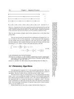
two small steps
big step
x
Figure 16.2.1. Step-doubling as a means for adaptive stepsize control in fourth-order Runge-Kutta.
Points where the derivative is evaluated are shown as filled circles. The open circle represents the same
derivatives as the filled circle immediately above it, so the total number of evaluations is 11 per two
steps. Comparing the accuracy of the big step with the two small steps gives a criterion for adjusting the
stepsize on the next step, or for rejecting the current step as inaccurate.
popularity of the classical fourth-order method: It seems to give the most bang
for the buck. However, Fehlberg discovered a fifth-order method with six function
evaluations where another combination of the six functions gives a fourth-order
method. The difference between the two estimates of y(x + h) can then be used as
an estimate of the truncation error to adjust the stepsize. Since Fehlberg’s original
formula, several other embedded Runge-Kutta formulas have been found.
Many practitioners were at one time wary of the robustness of Runge-Kutta-
Fehlberg methods. The feeling was that using the same evaluation points to advance
the function and to estimate the error was riskier than step-doubling, where the

error estimate is based on independent function evaluations. However, experience
has shown that this concern is not a problem in practice. Accordingly, embedded
Runge-Kutta formulas, which are roughly a factor of two more efficient, have
superseded algorithms based on step-doubling.
The general form of a fifth-order Runge-Kutta formula is
k
1
= hf(x
n
,y
n
)
k
2
=hf(x
n
+ a
2
h, y
n
+ b
21
k
1
)
···
k
6
=hf(x
n

+ a
6
h, y
n
+ b
61
k
1
+ ···+b
65
k
5
)
y
n+1
= y
n
+ c
1
k
1
+ c
2
k
2
+ c
3
k
3
+ c

4
k
4
+ c
5
k
5
+ c
6
k
6
+ O(h
6
)
(16.2.4)
The embedded fourth-order formula is
y
∗
n+1
= y
n
+ c
∗
1
k
1
+ c
∗
2
k

2
+ c
∗
3
k
3
+ c
∗
4
k
4
+ c
∗
5
k
5
+ c
∗
6
k
6
+ O(h
5
)(16.2.5)
and so the error estimate is
∆ ≡ y
n+1
− y
∗
n+1

=
6

i=1
(c
i
− c
∗
i
)k
i
(16.2.6)
The particular values of the various constants that we favor are those found by Cash
and Karp
[2]
, and given in the accompanying table. These give a more efficient
method than Fehlberg’s original values, with somewhat better error properties.
16.2 Adaptive Stepsize Control for Runge-Kutta
717
Sample page from NUMERICAL RECIPES IN C: THE ART OF SCIENTIFIC COMPUTING (ISBN 0-521-43108-5)
Copyright (C) 1988-1992 by Cambridge University Press.Programs Copyright (C) 1988-1992 by Numerical Recipes Software.
Permission is granted for internet users to make one paper copy for their own personal use. Further reproduction, or any copying of machine-
readable files (including this one) to any servercomputer, is strictly prohibited. To order Numerical Recipes books,diskettes, or CDROMs
visit website or call 1-800-872-7423 (North America only),or send email to (outside North America).
Cash-Karp Parameters for Embedded Runga-Kutta Method
i a
i
b
ij
c

i
c
∗
i
1
37
378
2825
27648
2
1
5
1
5
0 0
3
3
10
3
40
9
40
250
621
18575
48384
4
3
5
3

10
−
9
10
6
5
125
594
13525
55296
5 1 −
11
54
5
2
−
70
27
35
27
0
277
14336
6
7
8
1631
55296
175
512

575
13824
44275
110592
253
4096
512
1771
1
4
j =12345
Now that we know, at least approximately, what our error is, we need to
consider how to keep it within desired bounds. What is the relation between ∆
and h? According to (16.2.4) – (16.2.5), ∆ scales as h
5
. If we take a step h
1
and produce an error ∆
1
, therefore, the step h
0
that would have given some other
value ∆
0
is readily estimated as
h
0
= h
1





∆
0
∆
1




0.2
(16.2.7)
Henceforth we will let ∆
0
denote the desired accuracy. Then equation (16.2.7) is
used in two ways: If ∆
1
is larger than ∆
0
in magnitude, the equation tells how
much to decrease the stepsize when we retry the present (failed) step.If∆
1
is
smaller than ∆
0
, on the other hand, then the equation tells how much we can safely
increase the stepsize for the next step. Local extrapolation consists in accepting
the fifth order value y
n+1

, even though the error estimate actually applies to the
fourth order value y
∗
n+1
.
Our notation hides the fact that ∆
0
is actually a vector of desired accuracies,
one for each equation in the set of ODEs. In general, our accuracy requirement will
be that all equations are within their respective allowed errors. In other words, we
will rescale the stepsize according to the needs of the “worst-offender” equation.
How is ∆
0
, the desired accuracy, related to some looser prescription like “get a
solution good to one part in 10
6
”? That can be a subtle question, and it depends on
exactly what your application is! You may be dealing with a set of equations whose
dependent variables differ enormously in magnitude. In that case, you probably
want to use fractional errors, ∆
0
= y,whereis the number like 10
−6
or whatever.
On the other hand, you may have oscillatory functions that pass through zero but
are bounded by some maximum values. In that case you probably want to set ∆
0
equal to  times those maximum values.
A convenient way to fold these considerations into a generally useful stepper
routine is this: One of the arguments of the routine will of course be the vector of

dependent variables at the beginning of a proposed step. Call that y[1..n].Let
us require the user to specify for each step another, corresponding, vector argument
yscal[1..n], and also an overall tolerance level eps. Then the desired accuracy
718
Chapter 16. Integration of Ordinary Differential Equations
Sample page from NUMERICAL RECIPES IN C: THE ART OF SCIENTIFIC COMPUTING (ISBN 0-521-43108-5)
Copyright (C) 1988-1992 by Cambridge University Press.Programs Copyright (C) 1988-1992 by Numerical Recipes Software.
Permission is granted for internet users to make one paper copy for their own personal use. Further reproduction, or any copying of machine-
readable files (including this one) to any servercomputer, is strictly prohibited. To order Numerical Recipes books,diskettes, or CDROMs
visit website or call 1-800-872-7423 (North America only),or send email to (outside North America).
for the ith equation will be taken to be
∆
0
= eps × yscal[i] (16.2.8)
If you desire constant fractional errors, plug a pointer to y into the pointer to yscal
calling slot (no need to copy the values into a different array). If you desire constant
absolute errors relative to some maximum values, set the elements of yscal equal to
those maximum values. A useful “trick” for getting constant fractional errors except
“very” near zero crossings is to set yscal[i] equal to |y[i]| + |h × dydx[i]|.
(The routine odeint, below, does this.)
Here is a more technical point. We have to consider one additional possibility
for yscal. The error criteria mentioned thus far are “local,” in that they bound the
error of each step individually. In some applications you may be unusually sensitive
about a “global” accumulation of errors, from beginning to end of the integration
and in the worst possible case where the errors all are presumed to add with the
same sign. Then, the smaller the stepsize h, the smaller the value ∆
0
that you will
need to impose. Why? Because there will be more steps between your starting
and ending values of x. In such cases you will want to set yscal proportional to

h, typically to something like
∆
0
= h × dydx[i] (16.2.9)
This enforces fractional accuracy  not on thevalues of y but (much morestringently)
on the increments to those values at each step. But now look back at (16.2.7). If ∆
0
has an implicit scaling with h, then the exponent 0.20 is no longer correct: When
the stepsize is reduced from a too-large value, the new predicted value h
1
will fail to
meet the desired accuracy when yscal is also altered to this new h
1
value. Instead
of 0.20 = 1/5, we must scale by the exponent 0.25 = 1/4 for things to work out.
The exponents 0.20 and 0.25 are not really very different. This motivates us
to adopt the following pragmatic approach, one that frees us from having to know
in advance whether or not you, the user, plan to scale your yscal’s with stepsize.
Whenever we decrease a stepsize, let us use the larger value of the exponent (whether
we need it or not!), and whenever we increase a stepsize, let us use the smaller
exponent. Furthermore, because our estimates of error are not exact, but only
accurate to the leading order in h, we are advised to put in a safety factor S which is
a few percent smaller than unity. Equation (16.2.7) is thus replaced by
h
0
=










Sh
1




∆
0
∆
1




0.20
∆
0
≥ ∆
1
Sh
1





∆
0
∆
1




0.25
∆
0
< ∆
1
(16.2.10)
We have found this prescription to be a reliable one in practice.
Here, then, is a stepper program that takes one “quality-controlled” Runge-
Kutta step.