Tài liệu Integration of Ordinary Differential Equations part 5 pdf
Bạn đang xem bản rút gọn của tài liệu. Xem và tải ngay bản đầy đủ của tài liệu tại đây (206.74 KB, 9 trang )
724
Chapter 16. Integration of Ordinary Differential Equations
Sample page from NUMERICAL RECIPES IN C: THE ART OF SCIENTIFIC COMPUTING (ISBN 0-521-43108-5)
Copyright (C) 1988-1992 by Cambridge University Press.Programs Copyright (C) 1988-1992 by Numerical Recipes Software.
Permission is granted for internet users to make one paper copy for their own personal use. Further reproduction, or any copying of machine-
readable files (including this one) to any servercomputer, is strictly prohibited. To order Numerical Recipes books,diskettes, or CDROMs
visit website or call 1-800-872-7423 (North America only),or send email to (outside North America).
ym=vector(1,nvar);
yn=vector(1,nvar);
h=htot/nstep; Stepsize this trip.
for (i=1;i<=nvar;i++) {
ym[i]=y[i];
yn[i]=y[i]+h*dydx[i]; First step.
}
x=xs+h;
(*derivs)(x,yn,yout); Will use yout for temporary storage of deriva-
tives.h2=2.0*h;
for (n=2;n<=nstep;n++) { General step.
for (i=1;i<=nvar;i++) {
swap=ym[i]+h2*yout[i];
ym[i]=yn[i];
yn[i]=swap;
}
x+=h;
(*derivs)(x,yn,yout);
}
for (i=1;i<=nvar;i++) Last step.
yout[i]=0.5*(ym[i]+yn[i]+h*yout[i]);
free_vector(yn,1,nvar);
free_vector(ym,1,nvar);
}
CITED REFERENCES AND FURTHER READING:
Gear, C.W. 1971,
Numerical Initial Value Problems in Ordinary Differential Equations
(Englewood
Cliffs, NJ: Prentice-Hall),
§
6.1.4.
Stoer, J., and Bulirsch, R. 1980,
Introduction to Numerical Analysis
(New York: Springer-Verlag),
§
7.2.12.
16.4 Richardson Extrapolation and the
Bulirsch-Stoer Method
The techniques described in this section are not for differential equations
containing nonsmooth functions. For example, you might have a differential
equation whose right-handside involves a functionthat is evaluated by table look-up
and interpolation. If so, go back to Runge-Kutta with adaptive stepsize choice:
That method does an excellent job of feeling its way through rocky or discontinuous
terrain. It is also an excellent choice for quick-and-dirty, low-accuracy solution
of a set of equations. A second warning is that the techniques in this section are
not particularly good for differential equations that have singular points inside the
interval of integration. A regular solution must tiptoe very carefully across such
points. Runge-Kuttawithadaptivestepsize can sometimeseffect this;moregenerally,
there are special techniques available for such problems, beyond our scope here.
Apart from those two caveats, we believe that the Bulirsch-Stoer method,
discussed in this section, is the best known way to obtain high-accuracy solutions
to ordinary differential equations with minimal computational effort. (A possible
exception, infrequently encountered in practice, is discussed in §16.7.)
16.4 Richardson Extrapolation and the Bulirsch-Stoer Method
725
Sample page from NUMERICAL RECIPES IN C: THE ART OF SCIENTIFIC COMPUTING (ISBN 0-521-43108-5)
Copyright (C) 1988-1992 by Cambridge University Press.Programs Copyright (C) 1988-1992 by Numerical Recipes Software.
Permission is granted for internet users to make one paper copy for their own personal use. Further reproduction, or any copying of machine-
readable files (including this one) to any servercomputer, is strictly prohibited. To order Numerical Recipes books,diskettes, or CDROMs
visit website or call 1-800-872-7423 (North America only),or send email to (outside North America).
6 steps
2 steps
4 steps
⊗
extrapolation
to ∞ steps
x
x + H
y
Figure 16.4.1. Richardson extrapolation as used in the Bulirsch-Stoer method. A large interval H is
spanned by different sequences of finer and finer substeps. Their results are extrapolated to an answer
that is supposed to correspond to infinitely fine substeps. In the Bulirsch-Stoer method, the integrations
are done by the modified midpoint method, and the extrapolation technique is rational function or
polynomial extrapolation.
Three key ideas are involved. The first is Richardson’s deferred approach
to the limit, which we already met in §4.3 on Romberg integration. The idea is
to consider the final answer of a numerical calculation as itself being an analytic
function (if a complicated one) of an adjustable parameter like the stepsize h.That
analytic function can be probed by performing the calculation with various values
of h, none of them being necessarily small enough to yield the accuracy that we
desire. When we know enough about the function, we fit it to some analytic form,
and then evaluate it at that mythical and golden point h =0(see Figure 16.4.1).
Richardson extrapolation is a method for turning straw into gold! (Lead into gold
for alchemist readers.)
Thesecond ideahas to do withwhat kind offittingfunctionis used. Bulirschand
Stoer first recognized the strength of rational function extrapolation in Richardson-
type applications. That strength is to break the shackles of the power series and its
limited radius of convergence, outonly to the distance of the first pole in the complex
plane. Rational function fits can remain good approximations to analytic functions
even after the various terms in powers of h all have comparable magnitudes. In
other words, h can be so large as to make the whole notion of the “order” of the
method meaningless — and the method can still work superbly. Nevertheless, more
recent experience suggests that for smooth problems straightforward polynomial
extrapolation is slightly more efficient than rational function extrapolation. We will
accordingly adopt polynomial extrapolation as the default, but the routine bsstep
below allows easy substitution of one kind of extrapolation for the other. You
might wish at this point to review §3.1–§3.2, where polynomial and rational function
extrapolation were already discussed.
The third idea was discussed in the section before this one, namely to use
a method whose error function is strictly even, allowing the rational function or
polynomial approximation to be in terms of the variable h
2
instead of just h.
Put these ideas together and you have the Bulirsch-Stoer method
[1]
. A single
Bulirsch-Stoerstep takes us from x to x +H,whereHissupposed to be quite a large
726
Chapter 16. Integration of Ordinary Differential Equations
Sample page from NUMERICAL RECIPES IN C: THE ART OF SCIENTIFIC COMPUTING (ISBN 0-521-43108-5)
Copyright (C) 1988-1992 by Cambridge University Press.Programs Copyright (C) 1988-1992 by Numerical Recipes Software.
Permission is granted for internet users to make one paper copy for their own personal use. Further reproduction, or any copying of machine-
readable files (including this one) to any servercomputer, is strictly prohibited. To order Numerical Recipes books,diskettes, or CDROMs
visit website or call 1-800-872-7423 (North America only),or send email to (outside North America).
— not at all infinitesimal — distance. That single step is a grand leap consisting
of many (e.g., dozens to hundreds) substeps of modified midpoint method, which
are then extrapolated to zero stepsize.
The sequence of separate attempts to cross the interval H is made with
increasing values of n, the number of substeps. Bulirsch and Stoer originally
proposed the sequence
n =2,4,6,8,12, 16, 24, 32, 48, 64, 96,...,[n
j
=2n
j−2
],... (16.4.1)
More recent work by Deuflhard
[2,3]
suggests that the sequence
n =2,4,6,8,10, 12, 14,...,[n
j
=2j],... (16.4.2)
is usually more efficient. For each step, we do not know in advance how far up this
sequence we will go. After each successive n is tried, a polynomial extrapolation
is attempted. That extrapolation gives both extrapolated values and error estimates.
If the errors are not satisfactory, we go higher in n. If they are satisfactory, we go
on to the next step and begin anew with n =2.
Of course there must be some upper limit, beyond which we conclude that there
is some obstacle in our path in the interval H, so that we must reduce H rather than
just subdivide it more finely. In the implementations below, the maximum number
of n’s to be tried is called KMAXX. For reasons described below we usually take this
equal to 8; the 8th value of the sequence (16.4.2) is 16, so this is the maximum
number of subdivisions of H that we allow.
We enforce error control,as in the Runge-Kutta method, by monitoring internal
consistency, andadaptingstepsize tomatch a prescribed boundon thelocal truncation
error. Each new result from the sequence of modified midpoint integrations allows a
tableau like thatin §3.1 to be extended by one additional set of diagonals. The size of
the new correction added at each stage is taken as the (conservative) error estimate.
How should we use this error estimate to adjust the stepsize? The best strategy now
known is due to Deuflhard
[2,3]
. For completeness we describe it here:
Supposethe absolute value of the error estimate returnedfrom thekth column (andhence
the k +1st row) of the extrapolation tableau is
k+1,k
. Error control is enforced by requiring
k+1,k
< (16.4.3)
as the criterion for accepting the current step, where is the required tolerance. For the even
sequence (16.4.2) the order of the method is 2k +1:
k+1,k
∼ H
2k+1
(16.4.4)
Thus a simple estimate of a new stepsize H
k
toobtain convergenceinafixed column kwouldbe
H
k
= H
k+1,k
1/(2k+1)
(16.4.5)
Which column k should we aim to achieve convergence in? Let’s compare the work
required for different k. Suppose A
k
is the work to obtain row k of the extrapolation tableau,
so A
k+1
is the work to obtain column k. We will assume the work is dominated by the cost
of evaluating the functions defining the right-hand sides of the differential equations. For n
k
subdivisions in H, the number of function evaluations can be found from the recurrence
A
1
= n
1
+1
A
k+1
= A
k
+ n
k+1
(16.4.6)
16.4 Richardson Extrapolation and the Bulirsch-Stoer Method
727
Sample page from NUMERICAL RECIPES IN C: THE ART OF SCIENTIFIC COMPUTING (ISBN 0-521-43108-5)
Copyright (C) 1988-1992 by Cambridge University Press.Programs Copyright (C) 1988-1992 by Numerical Recipes Software.
Permission is granted for internet users to make one paper copy for their own personal use. Further reproduction, or any copying of machine-
readable files (including this one) to any servercomputer, is strictly prohibited. To order Numerical Recipes books,diskettes, or CDROMs
visit website or call 1-800-872-7423 (North America only),or send email to (outside North America).
The work per unit step to get column k is A
k+1
/H
k
, which we nondimensionalize with a
factor of H and write as
W
k
=
A
k+1
H
k
H (16.4.7)
= A
k+1
k+1,k
1/(2k+1)
(16.4.8)
The quantities W
k
can be calculated during the integration. The optimal column index q
is then defined by
W
q
=min
k=1,...,k
f
W
k
(16.4.9)
where k
f
is the final column, in which the error criterion (16.4.3) was satisfied. The q
determined from (16.4.9) defines the stepsize H
q
to be used as the next basic stepsize, so that
we can expect to get convergence in the optimal column q.
Two important refinements have to be made to the strategy outlined so far:
• If the current H is “too small,” then k
f
will be “too small,” and so q remains
“too small.” It may be desirable to increase H and aim for convergence in a
column q>k
f
.
•If the current H is “toobig,” we may not converge at all on the current step and we
will have to decrease H. We would like to detect this by monitoring the quantities
k+1,k
for each k so we can stop the current step as soon as possible.
Deuflhard’s prescription for dealing with these two problems uses ideas from communi-
cation theory to determine the “averageexpected convergence behavior” of the extrapolation.
His model produces certain correction factors α(k, q) by which H
k
is to be multiplied to try
to get convergence in column q. The factors α(k, q) depend only on and the sequence {n
i
}
and so can be computed once during initialization:
α(k, q)=
A
k+1
−A
q+1
(2k+1)(A
q+1
−A
1
+1)
for k<q (16.4.10)
with α(q, q)=1.
Now to handle the first problem, suppose convergence occurs in column q = k
f
.Then
rather than taking H
q
forthe nextstep,we might aim toincreasethestepsizetoget convergence
in column q +1. Since we don’t have H
q+1
available from the computation,we estimate it as
H
q+1
= H
q
α(q, q +1) (16.4.11)
By equation (16.4.7) this replacement is efficient, i.e., reduces the work per unit step, if
A
q+1
H
q
>
A
q+2
H
q+1
(16.4.12)
or
A
q+1
α(q, q +1)>A
q+2
(16.4.13)
During initialization, this inequality can be checked for q =1,2,...to determine k
max
,the
largest allowed column. Then when (16.4.12) is satisfied it will always be efficient to use
H
q+1
. (In practice we limit k
max
to8evenwhenis very small as there is very little further
gain in efficiency whereas roundoff can become a problem.)
The problem of stepsize reduction is handled by computing stepsize estimates
¯
H
k
≡ H
k
α(k,q),k=1,...,q−1(16.4.14)
during the current step. The
¯
H’s are estimates of the stepsize to get convergence in the
optimal column q.Ifany
¯
H
k
is “too small,” we abandon the current step and restart using
¯
H
k
. The criterion of being “too small” is taken to be
H
k
α(k, q +1)<H (16.4.15)
The α’s satisfy α(k, q +1) >α(k,q).
728
Chapter 16. Integration of Ordinary Differential Equations
Sample page from NUMERICAL RECIPES IN C: THE ART OF SCIENTIFIC COMPUTING (ISBN 0-521-43108-5)
Copyright (C) 1988-1992 by Cambridge University Press.Programs Copyright (C) 1988-1992 by Numerical Recipes Software.
Permission is granted for internet users to make one paper copy for their own personal use. Further reproduction, or any copying of machine-
readable files (including this one) to any servercomputer, is strictly prohibited. To order Numerical Recipes books,diskettes, or CDROMs
visit website or call 1-800-872-7423 (North America only),or send email to (outside North America).
During the first step, when we have no information about the solution, the stepsize
reduction check is made for all k. Afterwards, we test for convergence and for possible
stepsize reduction only in an “order window”
max(1,q−1) ≤ k ≤ min(k
max
,q+1) (16.4.16)
The rationale for the order window is that if convergence appears to occur for k<q−1it
is often spurious, resulting from some fortuitously small error estimate in the extrapolation.
On the other hand, if you need to go beyond k = q +1to obtain convergence, your local
model of the convergence behavior is obviously not very good and you need to cut the
stepsize and reestablish it.
In the routine bsstep, these various tests are actually carried out using quantities
(k) ≡
H
H
k
=
k+1,k
1/(2k+1)
(16.4.17)
called err[k] in the code. As usual, we include a “safety factor” in the stepsize selection.
This is implemented by replacing by 0.25. Other safety factors are explained in the
program comments.
Note that while the optimal convergence column is restricted to increase by at most one
on each step, a sudden drop in order is allowed by equation (16.4.9). This gives the method
a degree of robustness for problems with discontinuities.
Let us remind you once again that scaling of the variables is often crucial for
successful integration of differential equations. The scaling “trick” suggested in
the discussion following equation (16.2.8) is a good general purpose choice, but
not foolproof. Scaling by the maximum values of the variables is more robust, but
requires you to have some prior information.
The following implementation of a Bulirsch-Stoer step has exactly the same
calling sequence as the quality-controlled Runge-Kutta stepper rkqs. This means
that the driver odeint in §16.2 can be used for Bulirsch-Stoer as well as Runge-
Kutta: Just substitute bsstep for rkqs in odeint’s argument list. The routine
bsstep calls mmid to take the modified midpoint sequences, and calls pzextr,given
below, to do the polynomial extrapolation.
#include <math.h>
#include "nrutil.h"
#define KMAXX 8 Maximum row number used in the extrapola-
tion.#define IMAXX (KMAXX+1)
#define SAFE1 0.25 Safety factors.
#define SAFE2 0.7
#define REDMAX 1.0e-5 Maximum factor for stepsize reduction.
#define REDMIN 0.7 Minimum factor for stepsize reduction.
#define TINY 1.0e-30 Prevents division by zero.
#define SCALMX 0.1 1/SCALMX is the maximum factor by which a
stepsize can be increased.
float **d,*x;
Pointers to matrix and vector used by
pzextr
or
rzextr
.
void bsstep(float y[], float dydx[], int nv, float *xx, float htry, float eps,
float yscal[], float *hdid, float *hnext,
void (*derivs)(float, float [], float []))
Bulirsch-Stoer step with monitoring of local truncation error to ensure accuracy and adjust
stepsize. Input are the dependent variable vector
y[1..nv]
and its derivative
dydx[1..nv]
at the starting value of the independent variable
x
. Also input are the stepsize to be attempted
htry
, the required accuracy
eps
, and the vector
yscal[1..nv]
against which the error is
scaled. On output,
y
and
x
are replaced by their new values,
hdid
is the stepsize that was
actually accomplished, and
hnext
is the estimated next stepsize.
derivs
is the user-supplied
routine that computes the right-hand side derivatives. Be sure to set
htry
on successive steps