Tài liệu Laser điốt được phân phối thông tin phản hồi và các bộ lọc du dương quang P11 ppt

11
Other Wavelength Tunable Optical
Filters Based on the DFB Laser
Structure
11.1 INTRODUCTION
Optical tunable filters are key components of the future dense wavelength division
multiplexed (WDM) optical fibre networks. In such a network a number of information
channels are simultaneously transmitted through a single fibre by putting each channel on a
different optical carrier wavelength. The wavelength filter allows a single or multiple
channel(s) to be isolated at the receiving or routing node. The tunability of the filter allows
for dynamic network reconfiguration and increases versatility of the system. Ideally, the
wavelength filter should be tunable over the entire system bandwidth and should have no
secondary pass bands, or side lobes in its filter function.
WDM systems require optical tunable filters not only as channel selectors, but also as
post-optical-amplifier filters that reduce amplified spontaneous emission (ASE) noise [1].
Following the recent rapid advances in lightwave technology, wavelength tunable optical
filters are now incorporated in wavelength-division-multiplexed transmission systems to
increase the line capacity for lightwave telecommunication services. Optical filtering for
selection of channels separated by 2 nm is currently achievable, and narrower channel
separations may be possible as filter technologies improve. This would give more than a
hundred broadband channels in the low-loss fibre transmission region of 1.3 mm and/or
1.55 mm wavelength bands with each wavelength channel having a transmission bandwidth
of several gigahertz. Wavelength tunable optical filters have already been built into the
receiver for each subscriber in distribution networks [2]. Basically a semiconductor
wavelength tunable optical filter is a laser diode which is biased slightly below threshold.
When an optical signal of a wavelength close to the oscillation wavelength of the device is
incident upon the input, the signal is amplified and emitted at the output. By changing the
injection current, the wavelength can be tuned due to free carrier plasma and quantum
confined Stark effects.
Distributed feedback laser diode amplifiers (DFB LDAs) can be used as tunable wavelength
narrowband optical filters. This is because a DFB LDA has two main advantages:

single frequency with narrowband amplification and tunability of the lose gain profile
Distributed Feedback Laser Diodes and Optical Tunable Filters H. Ghafouri–Shiraz
# 2003 John Wiley & Sons, Ltd ISBN: 0-470-85618-1
maximum frequency by changing the amplifier’s bias current. DFB LDs have the advantage
of a single resonance at the centre of the stop band. Conventional uniform DFB LDs have
resonances on both sides of the stop band. This is, in general, a disadvantage since they may
oscillate at either of the two frequencies. Furthermore, the grating is less effective outside its
stop band. This drawback of index gratings has been overcome by inserting a =4 phase shift
at the centre of the structure [3–4]. In this way a resonance is produced at the centre of the
stop band. A passive index grating can perform useful filtering functions [5]. A DFB type
filter has the advantages of high gain and narrow bandwidth and disadvantages in that
the bandwidth and the transmissivity change with wavelength tuning.
Single-electrode wavelength tunable optical filters [6–8] have the problem of a changing
transmissivity during tuning. This is because the injection current of a single-electrode
device affects both the transmissivity and transmission wavelength. This problem has been
solved by employing a multi-electrode DFB filter which has more than one injection current
to control the gain and the central wavelength [9]. The tuning range of this filter is 33 GHz
with a constant gain and bandwidth. In 1992, Numai [10] reported the phase-controlled (PC)
DFB wavelength tunable optical filter. In this device the gain and transmission wavelength
were controlled independently by applying different injection currents. For this filter a
tuning range of 43 GHz (3.4 A
˚
) with constant gain of 27 dB and constant bandwidth of 0.4 A
˚
has been reported. The drawback of this filter is its very limited wavelength tuning range. In
general, to obtain a wider tuning range, suppression of the sub-modes is essential. To achieve
this goal, Numai [11] proposed the phase-shift-controlled (PSC) DFB filter where the side
modes were suppressed by the large gain margin when it was tuned around the Bragg
wavelength. This filter has a wider tuning range of 120 GHz (9.5 A
˚

) with constant gain of
24.5 dB and constant bandwidth of 12–13 GHz. In 1994, Tan et al. [12] proposed the
multiple-phase-shift-controlled distributed feedback wavelength tunable filter which has a
wavelength tuning range of about 30 A
˚
with side mode suppression ratio of more than 25 dB.
In this chapter we analyse the performance characteristics of DFB LD-based wavelength
tunable optical filters.
11.2 ANALYSIS
The analytical model for the filter structure is shown in Fig. 11.1. This filter consists of two
passive PC waveguides which control the transmission wavelength by changing the bias
Figure 11.1 Analytical model for the =4-phase-shifted double phase-shift-controlled wavelength
tunable filter.
286
OTHER WAVELENGTH TUNABLE OPTICAL FILTERS
current I
p
. Each PC section is sandwiched between two corrugated DFB active sections.
A =4 phase shift is also located at the centre of the middle DFB active section. The active
sections control the optical gain of the filter through the bias current I
a
. In the analysis we
have used the transfer matrix method to study the characteristics of this filter [4,13]. In doing
so, the filter cavity is divided into seven sections and the wave propagation in each section is
represented by a transfer matrix. Let us assume that the device has zero facet reflectivity and
the z-axis is along the filter cavity. The electric field EðzÞ within the filter cavity can be
expressed as
EðzÞ¼E
R
ðzÞþE

S
ðzÞ¼RðzÞ exp Àjb
o
zðÞþSðzÞ exp jb
o
zðÞ ð11:1Þ
where E
R
ðzÞ and E
S
ðzÞ are the normalised electric fields that propagate along opposite
directions, RðzÞ and SðzÞ are complex amplitudes of the forward and backward electric
fields, respectively, b
o
¼ p=L is the Bragg frequency of the grating and L is the grating
period. Substituting eqn (11.1) into Maxwell’s equations and neglecting the second
derivatives of both RðzÞ and SðzÞ with respect to z, as they are slowly varying functions of z,
we obtain the following pair of coupled mode equations [4,14]
dRðzÞ
dz
þ  À jðÞRðzÞ¼j SðzÞð11:2aÞ
dSðzÞ
dz
þ  À jðÞSðzÞ¼j RðzÞð11:2bÞ
In eqn (11.2) a is the mode gain per unit length, d ¼ b À b
o
is the detuning of the
propagation constant b from the Bragg propagation constant b
o
, and  is the grating

coupling coefficient. The filter structures used in this analysis are shown in Figs 11.1, 11.6,
11.9 and 11.15 where, for example in Fig. 11.1, I
a
and I
p
are the bias currents for the active
and phase-controlled sections, respectively, L
i
i ¼ 1; 6ðÞis the ith section length and
Z
j
j ¼ 1; 7ðÞis the jth position. In order to calculate the transmission characteristics of this
filter structure it is more convenient to use the transfer matrix method [4,13] where the cavity
is divided into seven sections. In each section we assume parameters ;  and  are uniform.
From the coupled wave equations, the transfer matrix which describes the propagating
electric field in the corrugated section between z
i
and z
iþ1
can be expressed as
E
R
z
iþ1
ðÞ
E
S
z
iþ1
ðÞ

!
¼
f
11
f
12
f
21
f
22
!
Á
E
R
z
i
ðÞ
E
S
z
i
ðÞ
!
¼ F
ðiÞ
Á
E
R
z
i

ðÞ
E
S
z
i
ðÞ
!
ð11:3Þ
where the matrix elements of matrix F
ðiÞ
are given as follows
f
11
¼
1
1 À 
2
i
E
i
À

2
i
E
i

exp Àjb
o
z

iþ1
À z
i
ðÞ½ ð11:4aÞ
f
12
¼
À
i
1 À 
2
i
E
i
À
1
E
i

exp Àjb
o
z
iþ1
þ z
i
ðÞ½ ð11:4bÞ
f
21
¼


i
1 À 
2
i
E
i
À
1
E
i

exp jb
o
z
iþ1
þ z
i
ðÞ½ ð11:4cÞ
f
22
¼
1
1 À 
2
i
1
E
i
À 
2

i
E
i

exp jb
o
z
iþ1
À z
i
ðÞ½ ð11:4dÞ
ANALYSIS
287
with
E
i
¼ exp g
i
z
iþ1
À z
i
ðÞ½ ð11:4eÞ

i
¼
j

i
À j

i
þ g
i
ð11:4fÞ
In the above equations g
i
is the complex propagation constant that satisfies the following
dispersion equation
g
2
i
¼ 
i
À j
i
ðÞ
2
þ
2
ð11:5Þ
On the other hand, since there is no active section and no grating in the planar phase-shift-
controlled (PSC) section (i.e. 
i
¼ 0 and 
i
¼ 0), the transfer matrix for the electric field of
this section is simplified to
E
R
z

iþ1
ðÞ
E
S
z
iþ1
ðÞ
!
¼
exp ðÞ 0
0 exp À ðÞ
!
E
R
z
i
ðÞ
E
S
z
i
ðÞ
!
¼ P
ðiÞ
E
R
z
i
ðÞ

E
S
z
i
ðÞ
!
ð11:6Þ
where ¼ g
p
L
p
À j
o
L
p
ÀÁ
, g
p
is the value of g
i
in the PSC section and L
p
is the length of
the PSC section. P
ðiÞ
is the corresponding transfer matrix of the PSC section. The amount of
phase shift, O, introduced by each PSC section is given by [11]
O ¼ Im 2g
p
L

p
ÀÁ
¼
4 n
a
À n
p
ÀÁ
L
p

B
ð11:7Þ
where I
m
means the imaginary part, n
a
and n
p
are the effective indices of the active and PC
sections, respectively. The value of n
p
decreases as the current injection into the PC section
increases, hence according to eqn (11.7) the value of O increases. The transfer matrix for
phase shift in the active section is given by
E
R
z
iþ1
ðÞ

E
S
z
iþ1
ðÞ
!
¼
exp jðÞ 0
0 exp ÀjðÞ
!
E
R
z
i
ðÞ
E
S
z
i
ðÞ
!
¼ S
E
R
z
i
ðÞ
E
S
z

i
ðÞ
!
ð11:8Þ
where  is the phase shift in the active section. By multiplying matrices representing the
planar phase-control sections, phase-shift section and the corrugated DFB sections together,
the overall transfer matrix for the structure shown in Figs 11.1 and 11.6 becomes
E
R
LðÞ
E
S
LðÞ
!
¼
T
11
T
12
T
21
T
22
!
E
R
0ðÞ
E
S
0ðÞ

!
¼ F
ð6Þ
PF
ð4Þ
SF
ð3Þ
PF
ð1Þ
E
R
0ðÞ
E
S
0ðÞ
!
ð11:9Þ
For the structures shown in Figs 11.9 and 11.15, respectively, eqn (11.9) becomes
E
R
LðÞ
E
S
LðÞ
!
¼
T
11
T
12

T
21
T
22
!
E
R
0ðÞ
E
S
0ðÞ
!
¼ F
ð5Þ
SF
ð4Þ
PF
ð2Þ
SF
ð1Þ
E
R
0ðÞ
E
S
0ðÞ
!
ð11:10Þ
288
OTHER WAVELENGTH TUNABLE OPTICAL FILTERS

and
E
R
LðÞ
E
S
LðÞ
!
¼
T
11
T
12
T
21
T
22
!
E
R
0ðÞ
E
S
0ðÞ
!
¼ F
ð7Þ
F
ð6Þ
F

ð5Þ
F
ð4Þ
F
ð3Þ
F
ð2Þ
F
ð1Þ
E
R
0ðÞ
E
S
0ðÞ
!
ð11:11Þ
In the above equation z
1
¼ 0 and in Figs 11.1, 11.6 and 11.15 z
7
¼ L, whereas z
6
¼ L in
Fig. 11.9. In an optical filter (such as the ones shown in Figs 11.1, 11.6, 11.9 and 11.15),
the power transmissivity, T, is defined as
T ¼
E
S
ðLÞ

E
R
ð0Þ








2
¼
1
T
22








2
ð11:12Þ
The threshold gain 
th
and the detuning parameter  can be obtained by solving the
following equation numerically

T
22

th
;Þ¼0ðð11:13Þ
The power transmissivity of the filter can be calculated by using the following expression
T ¼
1
T
22
 ¼ 0:98
th
;ðÞ








2
ð11:14Þ
In eqn (11.14), we have used  ¼ 0:98
th
[7] to achieve a higher output power and hence a
smaller 10 dB bandwidth.
11.3 RESULTS AND DISCUSSIONS OF VARIOUS OPTICAL
TUNABLE FILTERS
In this section we consider three different filter structures and analyse their performances.

11.3.1 A Quarter Wavelength Phase-shifted Double Phase-shift-controlled
DFB LD-based Wavelength Tunable Filter
In the following analysis we have used the total filter cavity length L ¼ 500 mm and the
lengths of PC sections L
2
¼ L
5
¼ 50 mm. The lengths of active sections which are optimised
to give maximum tuning range [15] are L
1
¼ 68:5 mm, L
3
¼ 37 mm, L
4
¼ 135 mm and
L
6
¼ 159:5 mm. Equation (11.13) has been solved numerically to analyse the filter structure
shown in Fig. 11.1. For a given value of , the numerical solution to eqn (11.13) gives
various oscillation modes for the device. The one having the lowest threshold gain is the
main mode. Sub-modes are the modes with larger threshold gains. The filter operates by
biasing the gain of the device slightly below the threshold gain of the main mode. The
normalised detuning coefficient of the main mode determines the amount of deviation of the
oscillation wavelength from the Bragg wavelength. The oscillation wavelength is the central
RESULTS AND DISCUSSIONS OF VARIOUS OPTICAL TUNABLE FILTERS
289
wavelength of the filter. For a given O the side mode suppression ratio (SMSR) is defined as
the ratio of the highest peak to the second highest peak of the filter power transmissivity. It
determines the amount of interference from the channel at the side mode wavelength. As the
central wavelength drifts away from the Bragg wavelength, the SMSR reduces. If the SMSR

is larger than 10 dB then the adjacent channel interference is minimal [7].
Figure 11.2 shows the calculated transmission spectra of the filter for various values of the
phase shift O ranging from 0 to 2 p. The horizontal axis is the relative wavelength defined as
 À 
B
where  is the operating wavelength of the filter, 
B
¼ 2 n
eff
Lð¼ 1:55 mm) is the
Bragg wavelength and n
eff
is the effective refractive index. The grating period and coupling
coefficient of 0:21 mm and 6 mm
À1
were used in this calculation. The figure clearly indicates
that as O increases the wavelength of the main mode shifts towards the shorter wavelength
side. The phase shift O can be controlled by changing the injection current I
p
of the PC
section. For example when I
p
increases, the effective refractive index n
p
decreases due to the
free carrier plasma effect and hence O increases according to eqn (11.7). When O ¼ 0or2p
(referred to as the stop band width of the filter, see case (a) in Fig. 11.2), the relative
wavelengths are at Æ12.5 A
˚
. This gives the filter wavelength tuning range of 25 A

˚
. The filter
peak gain varies between 34.9 and 36.1 dB with maximum deviation of 1.2 dB. The relative
wavelength is zero when O ¼ p (see case (l) in Fig. 11.2) and the filter SMSR ranges from
15.7 to 29.5 dB.
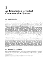
To investigate the effect of the grating period L on the filter performance we have
increased its value to 0:238 mm while the rest of the parameters remain identical to those in
Figure 11.2 Power transmissivity versus relative wavelength  À 
B
ðÞfor the following different
values of O. The parameters used are L
1
¼ 68:4 mm, L
2
¼ L
5
¼ 50 mm, L
3
¼ 36:98 mm,
L
4
¼ 135:02 mm, L
6
¼ 159:6 mm,  ¼ =2,  ¼ 6mm
À1
, L ¼ 0:21 mm and N ¼ 3:7. (a) O ¼ 0; 2;
(b) O ¼ 0:1; (c) O ¼ 0:2; (d) O ¼ 0:3; (e) O ¼ 0:4; (f) O ¼ 0:5; (g) O ¼ 0:6; (h) O ¼ 0:7;
(j) O ¼ 0:8; (k) O ¼ 0:9; (l) O ¼ ; (m) O ¼ 1:1; (n) O ¼ 1:2; (p) O ¼ 1:3; (q) O ¼ 1:4;
(r) O ¼ 1:5; (s) O ¼ 1:6; (t) O ¼ 1:7; (u) O ¼ 1:8; (v) O ¼ 1:9.
290

OTHER WAVELENGTH TUNABLE OPTICAL FILTERS
Fig. 11.2. The result is shown in Fig. 11.3. In this case when O ¼ 0or2p the relative
wavelengths are Æ14.15 A
˚
which gives the total filter tuning range of 28.3 A
˚
. This shows an
increase of 3.3 A
˚
compared with the filter shown in Fig. 11.2. The filter peak gain varies
between 35 and 36.1 dB and the filter SMSR ranges from 15 to 30 dB.
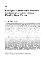
The effect of increasing  to 8 mm
À1
while keeping L ¼ 0:238 mm is shown in Fig. 11.4.
In this case the wavelength tuning range has increased to 31.1 A
˚
. The filter peak gain varies
between 33 and 35.2 dB and the SMSR ranges from 18.2 to 34.3 dB. These data indicate that
the deviation in the filter peak gain has increased to 2.2 dB compared with the previous two
cases. The filter spectra for the case where  ¼ 10 mm
À1
is shown in Fig. 11.5 where a
wavelength tuning range of 34.3 A
˚
has been achieved. The filter peak gain varies between
31.1 and 34.6 dB, which gives maximum deviation of 3.5 dB. The filter SMSR ranges from
19.6 to 34.7 dB.
We have also studied the performance characteristics of the filter structure shown in
Fig. 11.6 where the active sections have different grating coefficients. For example, the result
shown in Fig. 11.7 is for the case where 

1
¼ 6mm
À1
, 
2
¼ 4mm
À1
and L ¼ 0:21 mm. The
achieved peak filter gain varies between 35.6 and 36.4 dB, which gives 0.8 dB deviation. The
wavelength tuning range of the filter is 25.2 A
˚
and its SMSR ranges from 11.5 to 27 dB.
Figure 11.8 shows the case where 
1
¼ 4mm
À1
, 
2
¼ 6mm
À1
and L ¼ 0:21 mm. This filter
gives the wavelength tuning range of 24.4 A
˚
which is 0.8 A
˚
lower than that of Fig. 11.7.
Also, the SMSR ranges from 8.2 dB to 28.1 dB where the lower part is less than the
Figure 11.3 Power transmissivity versus relative wavelength  À 
B
ðÞfor the following different

values of O. The parameters used are L
1
¼ 68:4 mm, L
2
¼ L
5
¼ 50 mm, L
3
¼ 36:98 mm, L
4
¼
135:02 mm, L
6
¼ 159:6 mm,  ¼ =2,  ¼ 6mm
À1
, L ¼ 0:238 mm and N ¼ 3:2647. (a) O ¼ 0; 2; (b)
O ¼ 0:1; (c) O ¼ 0:2; (d) O ¼ 0:3; (e) O ¼ 0:4; (f) O ¼ 0:5; (g) O ¼ 0:6; (h) O ¼ 0:7;
(j) O ¼ 0:8; (k) O ¼ 0:9; (l) O ¼ ; (m) O ¼ 1:1; (n) O ¼ 1:2; (p) O ¼ 1:3; (q) O ¼ 1:4; (r)
O ¼ 1:5; (s) O ¼ 1:6; (t) O ¼ 1:7; (u) O ¼ 1:8; (v) O ¼ 1:9.
RESULTS AND DISCUSSIONS OF VARIOUS OPTICAL TUNABLE FILTERS
291