Tài liệu High Performance Computing on Vector Systems-P3 ppt

Over 10 TFLOPS Eigensolver on the Earth Simulator 53
Table 1. Hardware configuration, and the best performed applications of the ES (at
March, 2005)
The number of nodes 640 (8PE’s/node, total 5120PE’s)
PE VU(Mul/Add)×8pipes, Superscalar unit
Main memory & bandwidth 10TB (16GB/node), 256GB/s/node
Interconnection Metal-cable, Crossbar, 12.3GB/s/1way
Theoretical peak performance 40.96TFLOPS (64GFLOPS/node, 8GFLOPS/PE)
Linpack (TOP500 List) 35.86TFLOPS (87.5% of the peak) [7]
The fastest real application
26.58TFLOPS (64.9% of the peak) [8]
Complex number calculation (mainly FFT)
Our goal
Over 10TFLOPS (32.0% of the peak) [9]
Real number calculation (Numerical algebra)
3 Numerical Algorithms
The core of our program is to calculate the smallest eigenvalue and the corre-
sponding eigenvector for Hv = λv,wherethematrixisrealandsymmetric.Sev-
eral iterative numerical algorithms, i.e., the power method, the Lanczos method,
the conjugate gradient method (CG), and so on, are available. Since the ES is
public resource and a use of hundreds of nodes is limited, the most effective
algorithm must be selected before large-scale simulations.
3.1 Lanczos Method
The Lanczos method is one of the subspace projection methods that creates
a Krylov sequence and expands invariant subspace successively based on the
procedure of the Lanczos principle [10] (see Fig. 1(a)). Eigenvalues of the pro-
jected invariant subspace well approximate those of the original matrix, and the
subspace can be represented by a compact tridiagonal matrix. The main recur-
rence part of this algorithm repeats to generate the Lanczos vector v
i+1
from

v
i−1
and v
i
as seen in Fig. 1(a). In addition, an N-word buffer is required for
storing an eigenvector. Therefore, the memory requirement is 3N words.
As shown in Fig 1(a), the number of iterations depends on the input matrix,
however it is usually fixed by a constant number m. In the following, we choose
a smaller empirical fixed number i.e., 200 or 300, as an iteration count.
3.2 Preconditioned Conjugate Gradient Method
Alternative projection method exploring invariant subspace, the conjugate gra-
dient method is a popular algorithm, which is frequently used for solving linear
systems. The algorithm is shown in Fig. 1(b), which is modified from the original
algorithm [11] to reduce the load of the calculation S
A
. This method has a lot of
Please purchase PDF Split-Merge on www.verypdf.com to remove this watermark.
54 T. Imamura, S. Yamada, M. Machida
x
0
:= an initial guess.
β
0
:= 1,v
−1
:= 0,v
0
= x
0
/x

0

do i=0,1,..., m − 1,
or until β
i
<ǫ,
u
i
:= Hv
i
− β
i
v
i−1
α
i
:= (u
i
,v
i
)
w
i
:= u
i
− α
i
v
i
β

i
:= w
i

v
i+1
:= w
i
/β
i+1
enddo
x
0
:= an initial guess., p
0
:= 0,
x
0
:= x
0
/x
0
, X
0
:= Hx
0
,P
0
=0,
μ

−1
:= (x
0
,X
0
),w
0
:= X
0
− μ
−1
x
0
do i=0,1,..., until convergence
W
i
:= Hw
i
S
A
:= {w
i
,x
i
,p
i
}
T
{W
i

,X
i
,P
i
}
S
B
:= {w
i
,x
i
,p
i
}
T
{w
i
,x
i
,p
i
}
Solve the smallest eigenvalue μ
and the corresponding vector v,
S
A
v = μS
B
v, v =(α, β, γ)
T

.
μ
i
:= (μ +(x
i
,X
i
))/2
x
i+1
:= αw
i
+ βx
i
+ γp
i
,x
i+1
:= x
i+1
/x
i+1

p
i+1
:= αw
i
+ γp
i
,p

i+1
:= p
i+1
/p
i+1

X
i+1
:= αW
i
+ βX
i
+ γP
i
,X
i+1
:= X
i+1
/x
i+1

P
i+1
:= αW
i
+ γP
i
,P
i+1
:= P

i+1
/p
i+1

w
i+1
:= T (X
i+1
− μ
i
x
i+1
),w
i+1
:= w
i+1
/w
i+1

enddo
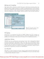
Fig. 1. The Lanczos algorithm (left (a)), and the preconditioned conjugate gradient
method (right (b))
advantages in the performance, because both the number of iterations and the
total CPU time drastically decrease depending on the preconditioning [11]. The
algorithm requires memory space to store six vectors, i.e., the residual vector w
i
,
the search direction vector p
i
, and the eigenvector x

i
,moreover,W
i
, P
i
,andX
i
.
Thus, the memory usage is totally 6N words.
In the algorithm illustrated in Fig. 1(b), an operator T indicates the precon-
ditioner. The preconditioning improves convergence of the CG method, and its
strength depends on mathematical characteristics of the matrix generally. How-
ever, it is hard to identify them in our case, because many unknown factor lies
in the Hamiltonian matrix. Here, we focus on the following two simple precondi-
tioners: point Jacobi, and zero-shift point Jacobi. The point Jacobi is the most
classical preconditioner, and it only operates the diagonal scaling of the matrix.
The zero-shift point Jacobi is a diagonal scaling preconditioner shifted by ‘μ
k
’
to amplify the eigenvector corresponding to the smallest eigenvalue, i.e., the pre-
Tabl e 2. Comparison among three preconditioners, and their convergence properties
1) NP 2) PJ 3) ZS-PJ
Num. of Iterations 268 133 91
Residual Error 1.445E-9 1.404E-9 1.255E-9
Elapsed Time [sec] 78.904 40.785 28.205
FLOPS 382.55G 383.96G 391.37G
Please purchase PDF Split-Merge on www.verypdf.com to remove this watermark.
Over 10 TFLOPS Eigensolver on the Earth Simulator 55
conditioning matrix is given by T =(D − μ
k

I)
−1
,whereμ
k
is the approximate
smallest eigenvalue which appears in the PCG iterations.
Table 2 summarizes a performance test of three cases, 1) without precondi-
tioner (NP), 2) point Jacobi (PJ), and 3) zero-shift point Jacobi (ZS-PJ) on the
ES, and the corresponding graph illustrates their convergence properties. Test
configuration is as follows; 1,502,337,600-dimensional Hamiltonian matrix (12
fermions on 20 sites) and we use 10 nodes of the ES. These results clearly reveal
that the zero-shift point Jacobi is the best preconditioner in this study.
4 Implementation on the Earth Simulator
The ES is basically classified in a cluster of SMP’s which are interconnected by
a high speed network switch, and each node comprises eight vector PE’s. In order
to achieve high performance in such an architecture, the intra-node parallelism,
i.e., thread parallelization and vectorization, is crucial as well as the inter-node
parallelization. In the intra-node parallel programming, we adopt the automatic
parallelization of the compiler system using a special language extension. In the
inter-node parallelization, we utilize the MPI library tuned for the ES. In this
section, we focus on a core operation Hv common for both the Lanczos and the
PCG algorithms and present the parallelization including data partitioning, the
communication, and the overlap strategy.
4.1 Core Operation: Matrix-Vector Multiplication
The Hubbard Hamiltonian H (1) is mathematically given as
H = I ⊗ A + A ⊗ I + D, (2)
where I, A,andD are the identity matrix, the sparse symmetric matrix due to
the hopping between neighboring sites, and the diagonal matrix originated from
the presence of the on-site repulsion, respectively.
Since the core operation Hv can be interpreted as a combination of the

alternating direction operations like the ADI method which appears in solving
a partial differential equation. In other word, it is transformed into the matrix-
matrix multiplications as Hv → (Dv, (I ⊗ A)v, (A ⊗ I)v) → (
¯
D ⊙ V,AV,V A
T
),
where the matrix V is derived from the vector v by a two-dimensional ordering.
The k-th element of the matrix D, d
k
, is also mapped onto the matrix
¯
D in the
same manner, and the operator ⊙ means an element-wise product.
4.2 Data Distribution, Parallel Calculation, and Communication
The matrix A, which represents the site hopping of up (or down) spin fermions,
is a sparse matrix. In contrast, the matrices V and
¯
D must be treated as dense
matrices. Therefore, while all the CRS (Compressed Row Storage) format of
Please purchase PDF Split-Merge on www.verypdf.com to remove this watermark.
56 T. Imamura, S. Yamada, M. Machida
the matrix A are stored on all the nodes, the matrices V and
¯
D are column-
wisely partitioned among all the computational nodes. Moreover, the row-wisely
partitioned V is also required on each node for parallel computing of VA
T
.This
means data re-distribution of the matrix V to V

T
, that is the matrix transpose,
and they also should be restored in the original distribution.
The core operation Hv including the data communication can be written as
follows:
CAL1: E
col
:=
¯
D
col
⊙ V
col
,
CAL2: W
col
1
:= E
col
+ AV
col
,
COM1: communication to transpose V
col
into V
row
,
CAL3: W
row
2

:= V
row
A
T
,
COM2: communication to transpose W
row
2
into W
col
2
,
CAL4: W
col
:= W
col
1
+ W
col
2
,
where the superscripts ‘col’ and ‘row’ denote column-wise and row-wise parti-
tioning, respectively.
The above operational procedure includes the matrix transpose twice which
normally requires all-to-all data communication. In the MPI standards, the all-
to-all data communication is realized by a collective communication function
MPI
Alltoallv. However, due to irregular and incontiguous structure of the
transferring data, furthermore strong requirement of a non-blocking property
(see following subsection), this communication must be composed of a point-

to-point or a one-side communication function. Probably it may sound funny
that MPI
Put is recommended by the developers [12]. However, the one-side
communication function MPI
Put works more excellently than the point-to-point
communication on the ES.
4.3 Communication Overlap
The MPI standard formally guarantees simultaneous execution of computation
and communication when it uses the non-blocking point-to-point communica-
tions and the one-side communications. This principally enables to hide the
communication time behind the computation time, and it is strongly believed
that this improves the performance. However, the overlap between communi-
cation and computation practically depends on an implementation of the MPI
library. In fact, the MPI library installed on the ES had not provided any func-
tions of the overlap until the end of March 2005, and the non-blocking MPI
Put
had worked as a blocking communication like MPI
Send. In the procedure of
the matrix-vector multiplication in Sect. 4.2, the calculations CAL1 and CAL2
and the communication COM1 are clearly found to be independently executed.
Moreover, although the relation between CAL3 and COM2 is not so simple,
the concurrent work can be realized in a pipelining fashion as shown in Fig. 2.
Thus, the two communication processes can be potentially hidden behind the
calculations.
Please purchase PDF Split-Merge on www.verypdf.com to remove this watermark.
Over 10 TFLOPS Eigensolver on the Earth Simulator 57
Node 0
Node 1
Node 2
Node 0 Node 1 Node 2

Node 0 Node 1 Node 2
→
T
VA
Synchronization
Calculation
Calculation
Calculation
→
T
VA
→
T
VA
Communication
Communication
Fig. 2. A data-transfer diagram to overlap
VA
T
(CAL3) with communication (COM2) in
acaseusingthreenodes
As mentioned in previous paragraph, MPI
Put installed on the ES prior to
the version March 2005 does not work as the non-blocking function
4
.Inimple-
mentation of our matrix-vector multiplication using the non-blocking MPI
Put
function, call of MPI
Win Fence to synchronize all processes is required in each

pipeline stage. Otherwise, two N-word communication buffers (for send and re-
ceive) should be retained until the completion of all the stages. On the other
hand, the completion of each stage is assured by return of the MPI Put in
the blocking mode, and send-buffer can be repeatedly used. Consequently, one
N-word communication buffer becomes free. Thus, we can adopt the blocking
MPI
Put to extend the maximum limit of the matrix size.
At a glance, this choice seems to sacrifice the overlap functionality of the MPI
library. However, one can manage to overlap computation with communication
even in the use of the blocking MPI
Put on the ES. The way is as follows: The
blocking MPI
Put can be assigned to a single PE per node by the intra-node
parallelization technique. Then, the assigned processor dedicates only the com-
munication task. Consequently, the calculation load is divided into seven PE’s.
This parallelization strategy, which we call task assignment (TA) method, im-
itates a non-blocking communication operation, and enables us to overlap the
blocking communication with calculation on the ES.
4.4 Effective Usage of Vector Pipelines, and Thread Parallelism
The theoretical FLOPS rate, F , in a single processor of the ES is calculated by
F =
4(#ADD + #MUL)
max{#ADD, #MUL, #VLD + #VST}
GFLOPS, (3)
4
The latest version supports both non-blocking and blocking modes.
Please purchase PDF Split-Merge on www.verypdf.com to remove this watermark.
58 T. Imamura, S. Yamada, M. Machida
where #ADD, #MUL, #VLD, #VST denote the number of additions, multipli-
cations, vector load, and store operations, respectively. According to the formula

(3), the performance of the matrix multiplications AV and VA
T
, described in the
previous section is normally 2.67 GFLOPS. However, higher order loop unrolling
decreases the number of VLD and VST instructions, and improves the perfor-
mance. In fact, when the degree of loop unrolling is 12 in the multiplication, the
performance is estimated to be 6.86 GFLOPS. Moreover,
• the loop fusion,
• the loop reconstruction,
• the efficient and novel vectorizing algorithms [13, 14],
• introduction of explicitly privatized variables (Fig. 3), and so on
improve the single node performance further.
4.5 Performance Estimation
In this section, we estimate the communication overhead and overall performance
of our eigenvalue solver.
First, let us summarize the notation of some variables. N basically means the
dimension of the system, however, in the matrix-representation the dimension
of matrix V becomes
√
N. P is the number of nodes, and in case of the ES
each node has 8 PE’s. In addition, data type is double precision floating point
number, and data size of a single word is 8 Byte.
As presented in previous sections, the core part of our code is the matrix-
vector multiplication in both the Lanczos and the PCG methods. We estimate
the message size issued on each node in the matrix-vector multiplication as
8N/P
2
[Byte]. From other work [12] which reports the network performance
of the ES, sustained throughput should be assumed 10[GB/s]. Since data com-
munication is carried 2P times, therefore, the estimated communication over-

head can be calculated 2P × (8N/P
2
[Byte])/(10[GB/s]) = 1.6N/P [nsec]. Next,
we estimate the computational cost. In the matrix-vector multiplication, about
40N/P flops are required on each node, and if sustained computational power
attains 8×6.8 [GFLOPS] (85% of the peak), the computational cost is estimated
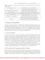
Fig. 3. An example code of loop reconstruction by introducing an explicitly privatized
variable. The modified code removes the loop-carried dependency of the variable nnx
Please purchase PDF Split-Merge on www.verypdf.com to remove this watermark.
Over 10 TFLOPS Eigensolver on the Earth Simulator 59
Fig. 4. More effective
communication hiding
technique, overlapping
much more vector opera-
tions with communication
on our TA method
(40N/P[flops])/(8 × 6.8[GFLOPS]) = 0.73N/P [nsec]. The estimated computa-
tional time is equivalent to almost half of the communication overhead, and it
suggests the peak performance of the Lanczos method, which considers no effect
from other linear algebra parts, is only less than 40% of the peak performance
of the ES (at the most 13.10TFLOPS on 512 nodes).
In order to reduce much more communication overhead, we concentrate on
concealing communication behind the large amounts of calculations by reorder-
ing the vector- and matrix-operations. As shown in Fig. 1(a), the Lanczos method
has strong dependency among vector- and matrix-operations, thus, we can not
find independent operations further. On the other hand, the PCG method con-
sists of a lot of vector operations, and some of them can work independently,
for example, inner-product (not including the term of W
i
) can perform with

the matrix-vector multiplications in parallel (see Fig. 4). In a rough estimation,
21N/P [flops] can be overlapped on each computational node, and half of the
idling time is removed from our code.
In deed, some results presented in previous sections apply the communication
hiding techniques shown here. One can easily understand that the performance
results of the PCG demonstrate the effect of reducing the communication over-
head. In Sect. 5, we examine our eigensolver on a lager partition on the ES, 512
nodes, which is the largest partition opened for non-administrative users.
5 Performance on the Earth Simulator
The performance of the Lanczos method and the PCG method with the TA
method for huge Hamiltonian matrices is presented in Table 3 and 4. Table 3
shows the system configurations, specifically, the numbers of sites and fermions
and the matrix dimension. Table 4 shows the performance of these methods on
512 nodes of the ES.
The total elapsed time and FLOPS rates are measured by using the built-
in performance analysis routine [15] installed on the ES. On the other hand,
the FLOPS rates of the solvers are evaluated by the elapsed time and the flops
count summed up by hand (the ratio of the computational cost per iteration
Please purchase PDF Split-Merge on www.verypdf.com to remove this watermark.
60 T. Imamura, S. Yamada, M. Machida
Tabl e 3. The dimension of Hamiltonian matrix H, the number of nodes, and memory
requirements. In case of the model 1 on the PCG method, memory requirement is
beyond 10TB
Model
No. of No. of Fermions Dimension No. of Memory [TB]
Sites (↑ / ↓ spin) of H Nodes Lanczos PCG
1 24 7/7 119,787,978,816 512 7.0 na
2 22 8/8 102,252,852,900 512 4.6 6.9
Tabl e 4. Performances of the Lanczos method and the PCG method on the ES (March
2005)

Lanczos method PCG method
Model
Itr.
Residual Elapsed time [sec]
Itr.
Residual Elapsed time [sec]
Error Total Solver Error Total Solver
1
200 5.4E-8
233.849 173.355
– –
– –
(TFLOPS) (10.215) (11.170) – –
2
300 3.6E-11
288.270 279.775
109 2.4E-9
68.079 60.640
(TFLOPS) (10.613) (10.906) (14.500) (16.140)
between the Lanczos and the PCG is roughly 2:3). As shown in Table 4, the
PCG method shows better convergence property, and it solves the eigenvalue
problems less than one third iteration of the Lanczos method. Moreover, con-
cerning the ratio between the elapsed time and flops count of both methods, the
PCG method performs excellently. It can be interpreted that the PCG method
overlaps communication with calculations much more effectively.
The best performance of the PCG method is 16.14TFLOPS on 512 nodes
which is 49.3% of the theoretical peak. On the other hand, Table 3 and 4 show
that the Lanczos method can solve up to the 120-billion-dimensional Hamiltonian
matrix on 512 nodes. To our knowledge, this size is the largest in the history of
the exact diagonalization method of Hamiltonian matrices.

6 Conclusions
The best performance, 16.14TFLOPS, of our high performance eigensolver is
comparable to those of other applications on the Earth Simulator as reported in
the Supercomputing conferences. However, we would like to point out that our
application requires massive communications in contrast to the previous ones.
We made many efforts to reduce the communication overhead by paying an at-
tention to the architecture of the Earth Simulator. As a result, we confirmed that
the PCG method shows the best performance, and drastically shorten the total
elapsed time. This is quite useful for systematic calculations like the present sim-
ulation code. The best performance by the PCG method and the world record of
Please purchase PDF Split-Merge on www.verypdf.com to remove this watermark.
Over 10 TFLOPS Eigensolver on the Earth Simulator 61
the large matrix operation are achieved. We believe that these results contribute
to not only Tera-FLOPS computing but also the next step of HPC, Peta-FLOPS
computing.
Acknowledgements
The authors would like to thank G. Yagawa, T. Hirayama, C. Arakawa, N. Inoue
and T. Kano for their supports, and acknowledge K. Itakura and staff members
in the Earth Simulator Center of JAMSTEC for their supports in the present cal-
culations. One of the authors, M.M., acknowledges T. Egami and P. Piekarz for
illuminating discussion about diagonalization for d-p model and H. Matsumoto
and Y. Ohashi for their collaboration on the optical-lattice fermion systems.
References
1. Machida M., Yamada S., Ohashi Y., Matsumoto H.: Novel Superfluidity in
a Trapped Gas of Fermi Atoms with Repulsive Interaction Loaded on an Opti-
cal Lattice. Phys. Rev. Lett., 93 (2004) 200402
2. Rasetti M. (ed.): The Hubbard Model: Recent Results. Series on Advances in
Statistical Mechanics, Vol. 7., World Scientific, Singapore (1991)
3. Montorsi A. (ed.): The Hubbard Model: A Collection of Reprints. World Scientific,
Singapore (1992)

4. Rigol M., Muramatsu A., Batrouni G.G., Scalettar R.T.: Local Quantum Critical-
ity in Confined Fermions on Optical Lattices. Phys. Rev. Lett., 91 (2003) 130403
5. Dagotto E.: Correlated Electrons in High-temperature Superconductors. Rev. Mod.
Phys., 66 (1994) 763
6. The Earth Simulator Center. />7. TOP500 Supercomputer Sites. />8. Shingu S. et al.: A 26.58 Tflops Global Atmospheric Simulation with the Spectral
Transform Method on the Earth Simulator. Proc. of SC2002, IEEE/ACM (2002)
9. Yamada S., Imamura T., Machida M.: 10TFLOPS Eigenvalue Solver for Strongly-
Correlated Fermions on the Earth Simulator. Proc. of PDCN2005, IASTED (2005)
10. Cullum J.K., Willoughby R.A.: Lanczos Algorithms for Large Symmetric Eigen-
value Computations, Vol. 1. SIAM, Philadelphia PA (2002)
11. Knyazev A.V.: Preconditioned Eigensolvers – An Oxymoron? Electr. Trans. on
Numer. Anal., Vol. 7 (1998) 104–123
12. Uehara H., Tamura M., Yokokawa M.: MPI Performance Measurement on the
Earth Simulator. NEC Research & Development, Vol. 44, No. 1 (2003) 75–79
13. Vorst H.A., Dekker K.: Vectorization of Linear Recurrence Relations. SIAM J. Sci.
Stat. Comput., Vol. 10, No. 1 (1989) 27–35
14. Imamura T.: A Group of Retry-type Algorithms on a Vector Computer. IPSJ,
Trans., Vol. 46, SIG 7 (2005) 52–62 (written in Japanese)
15. NEC Corporation, FORTRAN90/ES Programmerfs Guide, Earth Simulator Userfs
Manuals. NEC Corporation (2002)
Please purchase PDF Split-Merge on www.verypdf.com to remove this watermark.
Please purchase PDF Split-Merge on www.verypdf.com to remove this watermark.
First-Principles Simulation on Femtosecond
Dynamics in Condensed Matters Within
TDDFT-MD Approach
Yoshiyuki Miyamoto
∗
Fundamental and Environmental Research Laboratories, NEC Corp.,
34 Miyukigaoka, Tsukuba, 305-8501, Japan,

Abstract In this article, we introduce a new approach based on the time-dependent
density functional theory (TDDFT), where the real-time propagation of the Kohn-
Sham wave functions of electrons are treated by integrating the time-evolution opera-
tor. We have combined this technique with conventional classical molecular dynamics
simulation for ions in order to see very fast phenomena in condensed matters like as
photo-induced chemical reactions and hot-carrier dynamics. We briefly introduce this
technique and demonstrate some examples of ultra-fast phenomena in carbon nan-
otubes.
1 Introduction
In 1999, Professor Ahmed H. Zewail received the Nobel Prize in Chemistry for
his studies on transition states of chemical reaction using the femtosecond spec-
troscopy. (1 femtosecond (fs) = 10
−15
seconds.) This technique opened a door
to very fast phenomena in the typical time constant of hundreds fs. Meanwhile,
theoretical methods so-called as ab initio or first-principles methods, based on
time-independent Schr¨odinger equation, are less powerful to understand phe-
nomena within this time regime. This is because the conventional concept of the
thermal equilibrium or Fermi-Golden rule does not work and electron-dynamics
must be directly treated.
Density functional theory (DFT) [1] enabled us to treat single-particle rep-
resentation of electron wave functions in condensed matters even with many-
∗
The author is indebted to Professor Osamu Sugino for his great contribution in
developing the computer code “FPSEID” (´ef-ps´ai-d´ı:), which means First-Principles
Simulation tool for Electron Ion Dynamics. The MPI version of the FPSEID has
been developed with a help of Mr. Takeshi Kurimoto and CCRL MPI-team at NEC
Europe (Bonn). The researches on carbon nanotubes were done in collaboration
with Professors Angel Rubio and David Tom´anek. Most of the calculations were
performed by using the Earth Simulator with a help by Noboru Jinbo.

Please purchase PDF Split-Merge on www.verypdf.com to remove this watermark.
64 Y. Miyamoto
body interactions. This is owing to the theorem of one-to-one relationship be-
tween the charge density and the Hartree-exchange-correlation potential of elec-
trons. Thanks to this theorem, variational Euler equation of the total-energy
turns out to be Kohn-Sham equation [2], which is a DFT version of the time-
independent Schr¨odinger equation. Runge and Gross derived the time-dependent
Kohn-Sham equation [3] from the Euler equation of the “action” by extending
the one-to-one relationship into space and time. The usefulness of the time-
dependent DFT (TDDFT) [3] was demonstrated by Yabana and Bertsch [4],
who succeeded to improve the computed optical spectroscopy of finite systems
by Fourier-transforming the time-varying dipole moment initiated by a finite
replacement of electron clouds.
In this manuscript, we demonstrate that the use of TDDFT combined with
the molecular dynamics (MD) simulation is a powerful tool for approaching
the ultra-fast phenomena under electronic excitations [5]. In addition to the
‘real-time propagation’ of electrons [4], we treat ionic motion within Ehrenfest
approximation [6]. Since ion dynamics requires typical simulation time in the
order of hundreds fs, we need numerical stability in solving the time-dependent
Schr¨odinger equation for such a time constant. We chose the Suzuki-Trotter split
operator method [7], where an accuracy up to fourth order with respect to the
time-step dt is guaranteed. We believe that our TDDFT-MD simulations will be
verified by the pump-probe technique using the femtosecond laser.
The rest of this manuscript is organized as follows: In Sect. 2, we briefly ex-
plain how to perform the MD simulation under electronic excitation. In Sect. 3,
we present application of TDDFT-MD simulation for optical excitation and sub-
sequent dynamics in carbon nanotubes. We demonstrate two examples. The first
one is spontaneous emission of an oxygen (O) impurity atom from carbon nan-
otube, and the second one is rapid reduction of the energy gap of hot-electron
and hot-hole created in carbon nanotubes by optical excitation. In Sect. 4, we

summarize and present future aspects of the TDDFT simulations.
2 Computational Methods
In order to perform MD simulation under electronic excitation, electron dynam-
ics on real-time axis must be treated because of following reasons. The excited
state at particular atomic configuration can be mimicked by promoting electronic
occupation and solving the time-independent Schr¨odinger equation. However,
when atomic positions are allowed to move, level alternation among the states
with different occupation numbers often occurs. When the time-independent
Schr¨odinger equation is used throughout the MD simulation, the level assign-
ment is very hard and sometimes is made with mistake. On the other hand,
time-evolution technique by integrating the time-dependent Schr¨odinger equa-
tion enables us to know which state in current time originated from which state
in the past, so we can proceed MD simulation under the electronic excitation
with a substantial numerical stability.
Please purchase PDF Split-Merge on www.verypdf.com to remove this watermark.