Tài liệu High Performance Computing on Vector Systems-P9 pdf

Direct Numerical Simulation of Shear Flow Phenomena 241
u
y
0.25 0.5 0.75 1
-4
-2
0
2
4
v
y
0 0.001 0.002
-4
-2
0
2
4
ρ
y
0.998 1
-4
-2
0
2
4
T
y
1 1.002
-4
-2
0

2
4
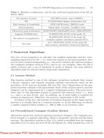
Fig. 14. Initial condition of the primitive variables u, v, ρ and T at the inflow x
0
=30
The initial condition of the mixing layer is provided by solving the steady
compressible two-dimensional boundary-layer equations. The initial coordinate
x
0
= 30 is chosen in a way that the vorticity thickness at the inflow is 1. By
that length scales are made dimensionless with δ. The spatial development of the
vorticity thickness of the boundary layer solution is shown in Fig. 13. Velocities
are normalized by U
∞
= U
1
and all other quantities by their values in the upper
stream. Figure 14 shows the initial values at x
0
= 30.
A cartesian grid of 2300 × 850 points in x-andy-direction is used. In stream-
wise direction the grid is uniform with spacing Δx =0.157 up to the sponge
region where the grid is highly stretched. In normal direction the grid is contin-
uously stretched with the smallest stepsize Δy =0.15 inside the mixing layer
(y = 0) and the largest spacing Δy =1.06 at the upper and lower boundaries.
In both directions smooth analytical functions are used to map the physical grid
on the computational equidistant grid. The grid and its decomposition into 8
domains is illustrated in Fig. 15.
4.2 Boundary Conditions
Non-reflective boundary conditions as described by Giles [7] are implemented

at the inflow and the freestream boundaries. To excite defined disturbances,
the flow is forced at the inflow using eigenfunctions from linear stability theory
(see Sect. 4.3) in accordance with the characteristic boundary condition. One-
dimensional characteristic boundary conditions posses low reflection coefficients
for low-amplitude waves as long as they impinge normal to the boundary. To
minimize reflections caused by oblique acoustic waves, a damping zone is applied
at the upper and lower boundary. It draws the flow variables Q to a steady state
solution Q
0
by modifying the time derivative obtained from the Navier-Stokes
Eqs. (3):
∂Q
∂t
=
∂Q
∂t
Navier-Stokes
− σ(y) · (Q − Q
0
) (32)
The spatial dependance of the damping term σ allows a smooth change from
no damping inside the flow field to maximum damping σ
max
at the boundaries.
Please purchase PDF Split-Merge on www.verypdf.com to remove this watermark.
242 A. Babucke et al.
Fig. 15. Grid in physical space showing every 25th gridline. Domain decomposition in
8 subdomains is indicated by red and blue colours
To avoid large structures passing the outflow, a combination of grid stretching
and low-pass filtering [9] is used as proposed by Colonius, Lele and Moin [3].

Disturbances become increasingly badly resolved as they propagate through the
sponge region and by applying a spatial filter, the perturbations are substantially
dissipated before they reach the outflow boundary. The filter is necessary to
avoid negative group velocities which occur when the non-dimensional modified
wavenumber k
∗
mod
is decreasing (see Fig. 1).
4.3 Linear Stability Theory
Viscous linear stability theory [10] describes the evolution of small amplitude
disturbances in a steady baseflow. It is used for forcing of the flow at the inflow
boundary. The disturbances have the form
Φ =
ˆ
Φ
(y)
· e
i(αx+γz−ωt)
+ c.c. (33)
with Φ =(u
′
,v
′
,w
′
,ρ
′
,T
′
,p

′
) representing the set of disturbances of the primitive
variables. The eigenfunctions are computed from the initial condition by com-
bining a matrix-solver and Wielandt iteration. The stability diagram in Fig. 16
shows the amplification rates at several x positions as a function of the fre-
quency ω. Note that negative values of −α
i
correspond to amplification while
positive values denote damping. Figure 16 shows that the highest amplification
Please purchase PDF Split-Merge on www.verypdf.com to remove this watermark.
Direct Numerical Simulation of Shear Flow Phenomena 243
Fig. 16. Stability diagram for 2d disturbances of the mixing layer showing the ampli-
fication rate −α
i
as a function of frequency ω and x-position
α
i
= −0.1122 is given for the fundamental frequency ω
0
=0.6296. Forcing at
the inflow is done using the eigenfunctions of the fundamental frequency ω
0
and
its subharmonics ω
0
/2, ω
0
/4andω
0
/8.

4.4 DNS Results
The high amplification rate as predicted by linear stability theory in the previous
Sect. 4.3 leads to a soon roll-up of the mixing layer. Further downstream, vortex
pairing takes place. Figure 17 illustrates the spatial development of the subsonic
mixing layer by showing the spanwise vorticity. In the center of Fig. 18 (−20 ≤
y ≤ 20) the spanwise vorticity is displayed. Above and below, the dilatation ∇u
gives an impression of the emitted sound. At the right side, the initial part of
the sponge zone is included. From the dilatation field, one can determine three
major sources of sound:
• in the initial part of the mixing layer (x = 50)
• in the area where vortex pairing takes place (x = 270)
• at the beginning of the sponge region
The first source corresponds to the fundamental frequency and is the strongest
source inside the flow field. Its position is upstream of the saturation of the
Please purchase PDF Split-Merge on www.verypdf.com to remove this watermark.
244 A. Babucke et al.
Fig. 17. Instantaneous view of the mixing layer showing roll-up of the vortices and
vortex pairing by plotting spanwise vorticity
Fig. 18. Instantaneous view of the mixing layer showing spanwise vorticity in the
center (−20 ≤ y ≤ 20) and dilatation to visualize the emitted sound. The beginning
of the outflow zone consisting of grid-stretching and filtering is indicated by a vertical
line
fundamental frequency which corresponds to the results of Colonius, Lele and
Moin [4]. The second source is less intensive and therefore can only be seen
by shading of the dilatation field. Source number three is directly related to the
sponge zone which indicates that dissipation of the vortices occurs to fast. Due to
that there is still the necessity to improve the combination of grid-stretching and
filtering. As dissipation inside the outflow region is depending on the timestep Δt,
Please purchase PDF Split-Merge on www.verypdf.com to remove this watermark.
Direct Numerical Simulation of Shear Flow Phenomena 245

choosing the appropriate combination of filter- and grid-stretching-parameters
is nontrivial.
5Performance
Good computational performance of a parallel code is first of all based on its
single processor performance. As the NEC SX-8 is a vector computer we use its
characteristic values for evaluation: the vector operation ratio is 99.75% and the
length of the vector pipe is 240 for a 2-d computation on a grid having 575 ×
425 points. Due to the fact that array sizes are already fixed at compilation,
optimized memory allocation is possible which reduces the bank conflict to 2%
of the total user time. All this results in a computational performance of 9548.6
MFLOP/s which corresponds to 60% of the peak performance of the NEC SX-
8 [14]. Computing 30000 timesteps required a user time of 5725 seconds, so one
timestep takes roughly 0.78 µs per grid-point.
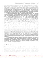
To evaluate the quality of the parallelization, speedup and efficiency are taken
into account. Again 30000 timesteps are computed and the grid size of each do-
main is those mentioned above. Figure 19 shows the dependance of speedup and
efficiency on the number of MPI processes. The efficiency decreases to 83% for
8 processes. A somehow strange behaviour is the fact that the efficiency of the
single processor run is less than one. Therefore efficiency is based on the maxi-
mum performance per processor. The reason for that is the non-exclusive usage
of a node for runs with less than 8 processors. So computational performance
can be affected by applications of other users. Comparing the achieved efficiency
of 89.3% for four processors with the theoretical value of 78.1% according to
Eq. (29) shows that even for 2-d computations, solving the tridiagonal equation
system is not the major part of computation.
If we extend the simulation to the three-dimensional case, Microtasking, the
second branch of the parallelization, is applied. We still use eight domains and by
# processors
MFLOP/s
efficency [%]

1 2 3 4 5 6 7 8
8000
8500
9000
9500
10000
50
60
70
80
90
100
performance
efficiency
Fig. 19. Computational
performance per proces-
sor (red) and efficiency
(blue) as a function of
MPI processes for 2-d
computations
Please purchase PDF Split-Merge on www.verypdf.com to remove this watermark.