Tài liệu 34 Iterative Image Restoration Algorithms pdf
Bạn đang xem bản rút gọn của tài liệu. Xem và tải ngay bản đầy đủ của tài liệu tại đây (312.97 KB, 20 trang )
Katsaggelos, A.K. “Iterative Image Restoration Algorithms”
Digital Signal Processing Handbook
Ed. Vijay K. Madisetti and Douglas B. Williams
Boca Raton: CRC Press LLC, 1999
c
1999byCRCPressLLC
34
Iterative Image Restoration
Algorithms
Aggelos K. Katsaggelos
Northwestern University
34.1 Introduction
34.2 Iterative Recovery Algorithms
34.3 Spatially Invariant Degradation
Degradation Model
•
Basic Iterative Restoration Algorithm
•
Convergence
•
Reblurring
34.4 Matrix-Vector Formulation
Basic Iteration
•
Least-Squares Iteration
34.5 Matrix-Vector and Discrete Frequency Representations
34.6 Convergence
Basic Iteration
•
Iteration with Reblurring
34.7 Use of Constraints
The Method of Projecting Onto Convex Sets (POCS)
34.8 Class of Higher Order Iterative Algorithms
34.9 Other Forms of
(x)
Ill-Posed Problems and Regularization Theory
•
Constrained
Minimization Regularization Approaches
•
Iteration Adap-
tive Image Restoration Algorithms
34.10 Discussion
References
34.1 Introduction
In this chapter we consider a class of iterative restoration algorithms. If y is the observed noisy and
blurred signal, D the operator describing the degradation system, x the input to the system, and n
the noise added to the output signal, the input-output relation is described by [3, 51]
y = Dx + n.
(34.1)
Henceforth, boldface lower-case letters represent vectors and boldface upper-case letters represent a
general operatoror a matrix. The problem, therefore, to be solvedis the inverse problem of recovering
x from knowledge of y, D, and n. Although the presentation will refer to and apply to signals of any
dimensionality, the restoration of greyscale images is the main application of interest.
There are numerous imaging applications which are described by Eq. (34.1)[3, 5, 28, 36, 52].
D, for example, might represent a model of the turbulent atmosphere in astronomical observations
with ground-based telescopes, or a model of the degradation introduced by an out-of-focus imaging
device. D might also represent the quantization performed on a signal, or a transformation of it, for
reducing the number of bits required to represent the signal (compression application).
c
1999 by CRC Press LLC
The success in solving any recovery problem depends on the amount of the available prior infor-
mation. This information refers to properties of the original signal, the degradation system (which
is in general only partially known), and the noise process. Such prior information can, for example,
be represented by the fact that the original signal is a sample of a stochastic field, or that the signal
is “smooth,” or that the signal takes only nonnegative values. Besides defining the amount of prior
information, the ease of incorporating it into the recovery algorithm is equally critical.
After the degradation model is established, the next step is the formulation of a solution approach.
This might involve the stochastic modeling of the input signal (and the noise), the determination
of the model parameters, and the formulation of a criterion to be optimized. Alternatively it might
involve the formulation of a functional to be optimized subject to constraints imposed by the prior
information. In the simplest possible case, the degradation equation defines directly the solution
approach. For example, if D is a square invertible matrix, and the noise is ignored in Eq. (34.1),
x = D
−1
y isthedesireduniquesolution. In most cases, however, the solution of Eq. (34.1)represents
an ill-posed problem[56]. Applicationofregularization theory transforms it to a well-posed problem
which provides meaningful solutions to the original problem.
There are a large number of approaches providing solutions to the image restoration problem. For
recent reviews of such approaches refer, for example, to [5, 28]. The intention of this chapter is to
concentrate only on a specific type of iterative algorithm, the successive approximation algorithm,
and its application to the signal and image restoration problem. The basic form of such an algorithm
is presented and analyzed first in detail to introduce the reader to the topic and address the issues
involved. More advanced forms of the algorithm are presented in subsequent sections.
34.2 Iterative Recovery Algorithms
Iterative algorithms form an important part of optimization theory and numerical analysis. They
date back at least to the Gauss years, but they also represent a topic of active research. A large
part of any textbook on optimization theory or numerical analysis deals with iterative optimization
techniques or algorithms [43, 44]. In this chapter we review certain iterative algorithms which have
been applied to solving specific signal recovery problems in the last 15 to 20 years. We will briefly
present some of the more basic algorithms and also review some of the recent advances.
Avery comprehensivepaperdescribingthevarious signal processinginverse problemswhichcan be
solvedbythesuccessiveapproximations iterativealgorithm isthepaper bySchaferetal. [49]. Thebasic
idea behind such an algorithm is that the solution to the problem of recovering a signal which satisfies
certain constraints from its degraded observation can be found by the alternate implementation
of the degradation and the constraint operator. Problems reported in [49] which can be solved
with such an iterative algorithm are the phase-only recovery problem, the magnitude-only recovery
problem, the bandlimitedextrapolation problem, the image restorationproblem, and the filterdesign
problem [10]. Reviews of iterative restoration algorithms are also presented in [7, 25]. There are
certain advantages associated with iterative restoration techniques, such as [25, 49]: (1) there is no
need to determine or implement the inverse of an operator; (2) knowledge about the solution can
be incorporated into the restoration process in a relatively straightforward manner; (3) the solution
process can be monitored as it progresses; and (4) the partially restored signal can be utilized in
determining unknown parameters pertaining to the solution.
In the following we first present the development and analysis of two simple iterative restoration
algorithms. Such algorithms are based on a simpler degradation model, when the degradation is
linear and spatially invariant, and the noise is ignored. The description of such algorithms is intended
to provide a good understanding of the various issues involved in dealing with iterative algorithms.
We then proceed to work with the matrix-vector representation of the degradation model and the
iterative algorithms. The degradation systems described now are linear but not necessarily spatially
c
1999 by CRC Press LLC
invariant. The relation between the matrix-vector and scalar representation of the degradation
equation and the iterative solution is also presented. Various forms of regularized solutions and the
resulting iterations are briefly presented. As it will become clear, the basic iteration is the basis for
any of the iterations to be presented.
34.3 Spatially Invariant Degradation
34.3.1 Degradation Model
Let us consider the following degradation model
y(i,j) = d(i,j) ∗ x(i, j) ,
(34.2)
where y(i,j) and x(i,j) represent, respectively, the observed degraded and original image, d(i,j)
the impulse response of the degradation system, and ∗ denotes two-dimensional (2D) convolution.
We rewrite Eq. (34.2)asfollows
(x(i, j)) = y(i,j) − d(i,j) ∗ x(i, j) = 0.
(34.3)
The restoration problem, therefore, of finding an estimate of x(i,j)given y(i, j)and d(i,j)becomes
the problem of finding a root of (x(i, j)) = 0.
34.3.2 Basic Iterative Restoration Algorithm
The following identity holds for any value of the parameter β
x(i,j) = x(i, j) + β
(
x(i,j)
)
.
(34.4)
Equation (34.4) forms the basis of the successive approximation iteration by interpreting x(i,j) on
the left-hand side as the solution at the current iteration step and x(i, j) on the right-hand side as
the solution at the previous iteration step. That is,
x
0
(i, j) = 0
x
k+1
(i, j) = x
k
(i, j) + β
(
x
k
(i, j)
)
= βy(i, j) +
(
δ(i, j) − βd(i, j )
)
∗ x
k
(i, j) ,
(34.5)
where δ(i, j) denotes the discrete delta function and β the relaxation parameter which controls the
convergence as well as the rate of convergence of the iteration. Iteration (34.5) is the basis of a
large number of iterative recovery algorithms, some of which will be presented in the subsequent
sections [1, 14, 17, 31, 32, 38]. This is the reason it will be analyzed in quite some detail. What
differentiates the various iterative algorithms is the form of the function (x(i, j)). Perhaps the
earliest reference to iteration (34.5) was by Van Cittert [61] in the 1930s. In this case the gain β was
equal to one. Jansson et al. [17] modified the Van Cittert algorithm by replacing β with a relaxation
parameter that depends on the signal. Also Kawata et al. [31, 32] used Eq. (34.5) for image restoration
with a fixed or a varying parameter β.
c
1999 by CRC Press LLC
34.3.3 Convergence
Clearly if a root of (x(i, j)) exists, this root is a fixed point of iteration (34.5), that is x
k+1
(i, j) =
x
k
(i, j). It is not guaranteed, however, that iteration (34.5)willconvergeevenifEq.(34.3) has
one or more solutions. Let us, therefore, examine under what conditions (sufficient conditions)
iteration (34.5) converges. Let us first rewrite it in the discrete frequency domain, by taking the 2D
discrete Fourier transform (DFT) of both sides. It should be mentioned here that the arrays involved
in iteration (34.5) are appropriately padded with zeros so that the result of 2D circular convolution
equals the result of 2D linear convolution in Eq. (34.2). The required padding by zeros determines
the size of the 2D DFT. Iteration (34.5) then becomes
X
0
(u, v) = 0
X
k+1
(u, v) = βY (u, v) +
(
1 − βD(u, v)
)
X
k
(u, v) ,
(34.6)
where X
k
(u, v), Y (u, v), and D(u, v) represent respectively the 2D DFT of x
k
(i, j), y(i, j), and
d(i,j), and (u, v) the discrete 2D frequency lattice. We express next X
k
(u, v) in terms of X
0
(u, v).
Clearly,
X
1
(u, v) = βY (u, v)
X
2
(u, v) = βY (u, v) +
(
1 − βD(u, v)
)
βY (u, v)
=
1
=0
(
1 − βD(u, v)
)
βY (u, v)
··· ·········
X
k
(u, v) =
k−1
=0
(
1 − βD(u, u)
)
βY (u, v)
=
1 −
(
1 − βD(u, v)
)
k
1 − (1 − βD(u, v))
βY (u, v)
=
(
1 −
(
1 − βD(u, v
))
k
)X(u, v)
(34.7)
if D(u, v) = 0.ForD(u, v) = 0,
X
k
(u, v) = k · βY (u, v) = 0,
(34.8)
since Y (u, v) = 0 at the discrete frequencies (u, v) for which D(u, v) = 0. Clearly, from Eq. (34.7)
if
|1 − βD(u, v)| < 1 ,
(34.9)
then
lim
k→∞
X
k
(u, v) = X(u, v) .
(34.10)
Having a closer look at the sufficient condition for convergence, Eq. (34.9), it can be rewritten as
|1 − βRe{D(u, v)}−βIm{D(u, v)}|
2
< 1
⇒
(
1 − βRe{D(u, v)}
)
2
+
(
βIm{D(u, v)}
)
2
< 1 .
(34.11)
Inequality (34.11) defines the region inside a circle of radius 1/β centered at c = (1/β, 0) in the
(Re{D(u, v)},Im{D(u, v)}) domain, as shown in Fig. 34.1. From this figure it is clear that the left
half-plane is not included in the region of convergence. That is, even though by decreasing β the size
c
1999 by CRC Press LLC
FIGURE 34.1: Geometric interpretation of the sufficient condition for convergence of the basic
iteration, where c = (1/β, 0).
of the region of convergence increases, if the real part of D(u, v) is negative, the sufficient condition
for convergence cannot be satisfied. Therefore, for the class of degradations that this is the case, such
as the degradation due to motion, iteration (34.5) is not guaranteed to converge.
The following form of (34.11) results when Im{D(u, v)}=0, which means that d(i,j) is sym-
metric
0 <β<
2
D
max
(u, v)
,
(34.12)
where D
max
(u, v) denotes the maximum value of D(u, v) over all frequencies (u, v). If we now also
take into account that d(i,j)is typically normalized, i.e.,
i,j
d(i,j) = 1, and represents a low pass
degradation, then D(0, 0) = D
max
(u, v) = 1. In this case (34.11) becomes
0 <β<2 .
(34.13)
From the above analysis, when the sufficient condition for convergence is satisfied, the iteration
convergestotheoriginal signal. Thisisalsotheinversesolutionobtaineddirectlyfromthe degradation
equation. That is, by rewriting Eq. (34.2) in the discrete frequency domain
Y (u, v) = D(u, v) · X(u, v) ,
(34.14)
we obtain, for D(u, v) = 0,
X(u, v) =
Y (u, v)
D(u, v)
.
(34.15)
Animportant pointtobemadehereis that, unlikethe iterative solution, the inversesolution(34.15)
can be obtained without imposing any requirements on D(u, v). That is, even if Eq. (34.2)or(34.14)
has a unique solution, that is, D(u, v) = 0 for all (u, v),iteration(34.5) may not converge if the
sufficient condition for convergence is not satisfied. It is not, therefore, the appropriate iteration
to solve the problem. Actually iteration (34.5) may not offer any advantages over the direct imple-
mentation of the inverse filter of Eq. (34.15) if no other features of the iterative algorithms are used,
as will be explained later. The only possible advantage of iteration (34.5)overEq.(34.15) is that
the noise amplification in the restored image can be controlled by terminating the iteration before
convergence, which represents another form of regularization. The effect of noise on the quality
of the restoration has been studied experimentally in [47]. An iteration which will converge to the
inverse solution of Eq. (34.2) for any d(i,j) is described in the next section.
c
1999 by CRC Press LLC
34.3.4 Reblurring
The degradation Eq. (34.2) can be modified so that the successive approximations iteration converges
for a larger class of degradations. That is, the observed data y(i, j) are first filtered (reblurred)
by a system with impulse response d
∗
(−i, −j),where
∗
denotes complex conjugation [33]. The
degradation Eq. (34.2), therefore, becomes
˜y(i,j) = y(i, j) ∗ d
∗
(−i, −j) = d
∗
(−i, −j)∗ d(i,j) ∗ x(i, j)
=
˜
d(i,j) ∗ x(i, j) .
(34.16)
If we follow the same steps as in the previous section substituting y(i,j) by ˜y(i, j) and d(i,j) by
˜
d(i,j) the iteration providing a solution to Eq. (34.16) becomes
x
0
(i, j) = 0
x
k+1
(i, j) = x
k
(i, j) + βd
∗
(−i, −j)∗ (y(i, j) − d(i, j) ∗ x
k
(i, j))
= βd
∗
(−i, −j)∗ y(i, j) + (δ(i, j )
− βd
∗
(−i, −j)∗ d(i,j)) ∗ x
k
(i, j) .
(34.17)
Now, the sufficient condition for convergence, corresponding to condition (34.9), becomes
|1 − β|D(u, v)|
2
| < 1 ,
(34.18)
which can be always satisfied for
0 <β<
2
max
u,v
|D(u, v)|
2
.
(34.19)
The presentation so far has followed a rather simple and intuitive path, hopefully demonstrating
some of the issues involved in developing and implementing an iterative algorithm. We move next to
the matrix-vector formulation of the degradation process and the restoration iteration. We borrow
results from numerical analysis in obtaining the convergence results of the previous section but also
more general results.
34.4 Matrix-Vector Formulation
What became clear from the previous sections is that in applying the successive approximations
iteration the restoration problem to be solved is brought first into the form of finding the root of
a function (see Eq. (34.3)). In other words, a solution to the restoration problem is sought which
satisfies
(x) = 0 ,
(34.20)
where x ∈ R
N
is the vector representation of the signal resulting from the stacking or ordering
of the original signal, and (x) represents a nonlinear in general function. The row-by-row from
left-to-right stacking of an image x(i, j) is typically referred to as lexicographic ordering.
Then the successive approximations iteration which might provide us with a solution to Eq. (34.20)
is given by
x
0
= 0
x
k+1
= x
k
+ β(x
k
)
= (x
k
).
(34.21)
c
1999 by CRC Press LLC
Clearly if x
∗
is a solution to (x) = 0, i.e., (x
∗
) = 0, then x
∗
is also a fixed point to the above
iteration since x
k+1
= x
k
= x
∗
. However, as was discussed in the previous section, even if x
∗
is
the unique solution to Eq. (34.20), this does not imply that iteration (34.21) will converge. This
again underlines the importance of convergence when dealing with iterative algorithms. The form
iteration (34.21) takes for various forms of the function (x) will be examined in the following
sections.
34.4.1 Basic Iteration
From the degradation Eq. (34.1), the simplest possible form (x) can take, when the noise is ignored,
is
(x) = y − Dx .
(34.22)
Then Eq. (34.21) becomes
x
0
= 0
x
k+1
= x
k
+ β(y − Dx
k
)
= βy + (I − βD)x
k
= βy + G
1
x
k
,
(34.23)
where I is the identity operator.
34.4.2 Least-Squares Iteration
A least-squares approach can be followed in solving Eq. (34.1). That is, a solution is sought which
minimizes
M(x) =y − Dx
2
.
(34.24)
A necessary condition for M(x) to have a minimum is that its gradient with respect to x is equal to
zero, which results in the normal equations
D
T
Dx = D
T
y
(34.25)
or
(x) = D
T
(y − Dx) = 0 ,
(34.26)
where
T
denotes the transpose of a matrix or vector. Application of iteration (34.21) then results in
x
0
= 0
x
k+1
= x
k
+ βD
T
(y − Dx
k
)
= βD
T
y + (I − βD
T
D)x
k
= βD
T
y + G
2
x
k
.
(34.27)
It is mentioned here that the matrix-vector representation of an iteration does not necessarily
determine the way the iteration is implemented. In other words, the pointwise version of the iteration
may be more efficient from the implementation point of view than the matrix-vector form of the
iteration.
c
1999 by CRC Press LLC