Ogata modern control engineering 5th txtbk

www.TheSolutionManual.com



www.TheSolutionManual.com

Modern Control
Engineering
Fifth Edition
Katsuhiko Ogata

Prentice Hall
Boston Columbus Indianapolis New York San Francisco Upper Saddle River
Amsterdam Cape Town Dubai London Madrid Milan Munich Paris Montreal Toronto
Delhi Mexico City Sao Paulo Sydney Hong Kong Seoul Singapore Taipei Tokyo


www.TheSolutionManual.com

VP/Editorial Director, Engineering/Computer Science: Marcia J. Horton
Assistant/Supervisor: Dolores Mars
Senior Editor: Andrew Gilfillan
Associate Editor: Alice Dworkin
Editorial Assistant: William Opaluch
Director of Marketing: Margaret Waples
Senior Marketing Manager: Tim Galligan
Marketing Assistant: Mack Patterson
Senior Managing Editor: Scott Disanno
Art Editor: Greg Dulles
Senior Operations Supervisor: Alan Fischer
Operations Specialist: Lisa McDowell

Art Director: Kenny Beck
Cover Designer: Carole Anson
Media Editor: Daniel Sandin

Credits and acknowledgments borrowed from other sources and reproduced, with permission, in this
textbook appear on appropriate page within text.
MATLAB is a registered trademark of The Mathworks, Inc., 3 Apple Hill Drive, Natick MA 01760-2098.
Copyright © 2010, 2002, 1997, 1990, 1970 Pearson Education, Inc., publishing as Prentice Hall, One Lake
Street, Upper Saddle River, New Jersey 07458. All rights reserved. Manufactured in the United States of
America. This publication is protected by Copyright, and permission should be obtained from the publisher
prior to any prohibited reproduction, storage in a retrieval system, or transmission in any form or by any
means, electronic, mechanical, photocopying, recording, or likewise. To obtain permission(s) to use material
from this work, please submit a written request to Pearson Education, Inc., Permissions Department, One
Lake Street, Upper Saddle River, New Jersey 07458.
Many of the designations by manufacturers and seller to distinguish their products are claimed as
trademarks. Where those designations appear in this book, and the publisher was aware of a trademark
claim, the designations have been printed in initial caps or all caps.
Library of Congress Cataloging-in-Publication Data on File

10 9 8 7 6 5 4 3 2 1

ISBN 10: 0-13-615673-8
ISBN 13: 978-0-13-615673-4


www.TheSolutionManual.com

C
Contents

Preface
Chapter 1
1–1
1–2
1–3
1–4
1–5

2–6

Introduction to Control Systems

1

Introduction
1
Examples of Control Systems
4
Closed-Loop Control Versus Open-Loop Control
7
Design and Compensation of Control Systems
9
Outline of the Book
10

Chapter 2
2–1
2–2
2–3
2–4

2–5

ix

Mathematical Modeling of Control Systems

Introduction
13
Transfer Function and Impulse-Response Function
15
Automatic Control Systems
17
Modeling in State Space
29
State-Space Representation of Scalar Differential
Equation Systems
35
Transformation of Mathematical Models with MATLAB

13

39

iii


www.TheSolutionManual.com
2–7

Linearization of Nonlinear Mathematical Models

Example Problems and Solutions
Problems

Chapter 3

60

Mathematical Modeling of Mechanical Systems
and Electrical Systems

Introduction

3–2

Mathematical Modeling of Mechanical Systems

3–3

Mathematical Modeling of Electrical Systems
Problems

63
72

86

97

Mathematical Modeling of Fluid Systems
and Thermal Systems

4–1

Introduction

4–2

Liquid-Level Systems

4–3

Pneumatic Systems

106

4–4

Hydraulic Systems

123

4–5

Thermal Systems
Problems

101

136
140

152

Transient and Steady-State Response Analyses

5–1

Introduction

5–2

First-Order Systems

5–3

Second-Order Systems

164

5–4

Higher-Order Systems

179

5–5

Transient-Response Analysis with MATLAB

5–6

Routh’s Stability Criterion

5–7

Effects of Integral and Derivative Control Actions
on System Performance
218

5–8

Steady-State Errors in Unity-Feedback Control Systems
Problems

159

159
161

263

183

212

Example Problems and Solutions

Contents

100

100

Example Problems and Solutions

Chapter 5

63

63

Example Problems and Solutions

iv

46

3–1

Chapter 4

43

231

225


www.TheSolutionManual.com
Chapter 6

Control Systems Analysis and Design
by the Root-Locus Method

6–1

Introduction

6–2

Root-Locus Plots

6–3

Plotting Root Loci with MATLAB

6–4

Root-Locus Plots of Positive Feedback Systems

6–5

Root-Locus Approach to Control-Systems Design

6–6

Lead Compensation

6–7

Lag Compensation

6–8

Lag–Lead Compensation

6–9

Parallel Compensation

269
270

Chapter 7

290
303
308

311
321
330
342

Example Problems and Solutions
Problems

269

347

394

Control Systems Analysis and Design by the
Frequency-Response Method

7–1

Introduction

7–2

Bode Diagrams

7–3

Polar Plots

7–4

Log-Magnitude-versus-Phase Plots

7–5

Nyquist Stability Criterion

7–6

Stability Analysis

7–7

Relative Stability Analysis

7–8

Closed-Loop Frequency Response of Unity-Feedback
Systems
477

7–9

Experimental Determination of Transfer Functions

398
403

427
443

445

454
462

486

7–10 Control Systems Design by Frequency-Response Approach
7–11 Lead Compensation
7–12 Lag Compensation

502
511

Example Problems and Solutions

Chapter 8

521

561

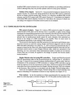
PID Controllers and Modified PID Controllers

8–1

Introduction

8–2

Ziegler–Nichols Rules for Tuning PID Controllers

Contents

491

493

7–13 Lag–Lead Compensation
Problems

398

567

567
568
v


www.TheSolutionManual.com
8–3
8–4
8–5
8–6
8–7

Design of PID Controllers with Frequency-Response
Approach
577
Design of PID Controllers with Computational Optimization
Approach
583
Modifications of PID Control Schemes
590
Two-Degrees-of-Freedom Control
592
Zero-Placement Approach to Improve Response
Characteristics
595

Example Problems and Solutions
614
Problems

Chapter 9
9–1
9–2
9–3
9–4
9–5
9–6
9–7

Control Systems Analysis in State Space

Chapter 10

vi

648

Introduction
648
State-Space Representations of Transfer-Function
Systems
649
Transformation of System Models with MATLAB
656
Solving the Time-Invariant State Equation
660

Some Useful Results in Vector-Matrix Analysis
668
Controllability
675
Observability
682
Example Problems and Solutions
688
Problems

10–1
10–2
10–3
10–4
10–5
10–6
10–7
10–8
10–9

641

720

Control Systems Design in State Space

Introduction
722
Pole Placement
723

Solving Pole-Placement Problems with MATLAB
735
Design of Servo Systems
739
State Observers
751
Design of Regulator Systems with Observers
778
Design of Control Systems with Observers
786
Quadratic Optimal Regulator Systems
793
Robust Control Systems
806
Example Problems and Solutions
817
Problems
855

Contents

722


www.TheSolutionManual.com
Appendix A

Laplace Transform Tables

859

Appendix B

Partial-Fraction Expansion

867

Appendix C

Vector-Matrix Algebra

874

References

882

Index

886

Contents

vii


www.TheSolutionManual.com

This page intentionally left blank

www.TheSolutionManual.com

P
Preface

This book introduces important concepts in the analysis and design of control systems.
Readers will find it to be a clear and understandable textbook for control system courses
at colleges and universities. It is written for senior electrical, mechanical, aerospace, or
chemical engineering students. The reader is expected to have fulfilled the following
prerequisites: introductory courses on differential equations, Laplace transforms, vectormatrix analysis, circuit analysis, mechanics, and introductory thermodynamics.
The main revisions made in this edition are as follows:
• The use of MATLAB for obtaining responses of control systems to various inputs
has been increased.
• The usefulness of the computational optimization approach with MATLAB has been
demonstrated.
• New example problems have been added throughout the book.
• Materials in the previous edition that are of secondary importance have been deleted
in order to provide space for more important subjects. Signal flow graphs were
dropped from the book. A chapter on Laplace transform was deleted. Instead,
Laplace transform tables, and partial-fraction expansion with MATLAB are presented in Appendix A and Appendix B, respectively.
• A short summary of vector-matrix analysis is presented in Appendix C; this will help
the reader to find the inverses of n x n matrices that may be involved in the analysis and design of control systems.
This edition of Modern Control Engineering is organized into ten chapters.The outline of
this book is as follows: Chapter 1 presents an introduction to control systems. Chapter 2
ix


www.TheSolutionManual.com
deals with mathematical modeling of control systems. A linearization technique for nonlinear mathematical models is presented in this chapter. Chapter 3 derives mathematical

models of mechanical systems and electrical systems. Chapter 4 discusses mathematical
modeling of fluid systems (such as liquid-level systems, pneumatic systems, and hydraulic
systems) and thermal systems.
Chapter 5 treats transient response and steady-state analyses of control systems.
MATLAB is used extensively for obtaining transient response curves. Routh’s stability
criterion is presented for stability analysis of control systems. Hurwitz stability criterion
is also presented.
Chapter 6 discusses the root-locus analysis and design of control systems, including
positive feedback systems and conditionally stable systems Plotting root loci with MATLAB is discussed in detail. Design of lead, lag, and lag-lead compensators with the rootlocus method is included.
Chapter 7 treats the frequency-response analysis and design of control systems. The
Nyquist stability criterion is presented in an easily understandable manner.The Bode diagram approach to the design of lead, lag, and lag-lead compensators is discussed.
Chapter 8 deals with basic and modified PID controllers. Computational approaches
for obtaining optimal parameter values for PID controllers are discussed in detail, particularly with respect to satisfying requirements for step-response characteristics.
Chapter 9 treats basic analyses of control systems in state space. Concepts of controllability and observability are discussed in detail.
Chapter 10 deals with control systems design in state space. The discussions include
pole placement, state observers, and quadratic optimal control. An introductory discussion of robust control systems is presented at the end of Chapter 10.
The book has been arranged toward facilitating the student’s gradual understanding
of control theory. Highly mathematical arguments are carefully avoided in the presentation of the materials. Statement proofs are provided whenever they contribute to the
understanding of the subject matter presented.
Special effort has been made to provide example problems at strategic points so that
the reader will have a clear understanding of the subject matter discussed. In addition,
a number of solved problems (A-problems) are provided at the end of each chapter,
except Chapter 1. The reader is encouraged to study all such solved problems carefully;
this will allow the reader to obtain a deeper understanding of the topics discussed. In
addition, many problems (without solutions) are provided at the end of each chapter,
except Chapter 1. The unsolved problems (B-problems) may be used as homework or
quiz problems.
If this book is used as a text for a semester course (with 56 or so lecture hours), a good
portion of the material may be covered by skipping certain subjects. Because of the
abundance of example problems and solved problems (A-problems) that might answer

many possible questions that the reader might have, this book can also serve as a selfstudy book for practicing engineers who wish to study basic control theories.
I would like to thank the following reviewers for this edition of the book: Mark Campbell, Cornell University; Henry Sodano, Arizona State University; and Atul G. Kelkar,
Iowa State University. Finally, I wish to offer my deep appreciation to Ms.Alice Dworkin,
Associate Editor, Mr. Scott Disanno, Senior Managing Editor, and all the people involved in this publishing project, for the speedy yet superb production of this book.
Katsuhiko Ogata
x

Preface


www.TheSolutionManual.com

1
Introduction
to Control Systems

1–1 INTRODUCTION
Control theories commonly used today are classical control theory (also called conventional control theory), modern control theory, and robust control theory. This book
presents comprehensive treatments of the analysis and design of control systems based
on the classical control theory and modern control theory.A brief introduction of robust
control theory is included in Chapter 10.
Automatic control is essential in any field of engineering and science. Automatic
control is an important and integral part of space-vehicle systems, robotic systems, modern manufacturing systems, and any industrial operations involving control of temperature, pressure, humidity, flow, etc. It is desirable that most engineers and scientists are
familiar with theory and practice of automatic control.
This book is intended to be a text book on control systems at the senior level at a college or university. All necessary background materials are included in the book. Mathematical background materials related to Laplace transforms and vector-matrix analysis
are presented separately in appendixes.
Brief Review of Historical Developments of Control Theories and Practices.
The first significant work in automatic control was James Watt’s centrifugal governor for the speed control of a steam engine in the eighteenth century. Other
significant works in the early stages of development of control theory were due to

1


www.TheSolutionManual.com
Minorsky, Hazen, and Nyquist, among many others. In 1922, Minorsky worked on
automatic controllers for steering ships and showed how stability could be determined from the differential equations describing the system. In 1932, Nyquist
developed a relatively simple procedure for determining the stability of closed-loop
systems on the basis of open-loop response to steady-state sinusoidal inputs. In 1934,
Hazen, who introduced the term servomechanisms for position control systems,
discussed the design of relay servomechanisms capable of closely following a changing input.
During the decade of the 1940s, frequency-response methods (especially the Bode
diagram methods due to Bode) made it possible for engineers to design linear closedloop control systems that satisfied performance requirements. Many industrial control
systems in 1940s and 1950s used PID controllers to control pressure, temperature, etc.
In the early 1940s Ziegler and Nichols suggested rules for tuning PID controllers, called
Ziegler–Nichols tuning rules. From the end of the 1940s to the 1950s, the root-locus
method due to Evans was fully developed.
The frequency-response and root-locus methods, which are the core of classical control theory, lead to systems that are stable and satisfy a set of more or less arbitrary performance requirements. Such systems are, in general, acceptable but not optimal in any
meaningful sense. Since the late 1950s, the emphasis in control design problems has been
shifted from the design of one of many systems that work to the design of one optimal
system in some meaningful sense.
As modern plants with many inputs and outputs become more and more complex,
the description of a modern control system requires a large number of equations. Classical control theory, which deals only with single-input, single-output systems, becomes
powerless for multiple-input, multiple-output systems. Since about 1960, because the
availability of digital computers made possible time-domain analysis of complex systems, modern control theory, based on time-domain analysis and synthesis using state
variables, has been developed to cope with the increased complexity of modern plants
and the stringent requirements on accuracy, weight, and cost in military, space, and industrial applications.
During the years from 1960 to 1980, optimal control of both deterministic and stochastic systems, as well as adaptive and learning control of complex systems, were fully
investigated. From 1980s to 1990s, developments in modern control theory were centered around robust control and associated topics.
Modern control theory is based on time-domain analysis of differential equation
systems. Modern control theory made the design of control systems simpler because

the theory is based on a model of an actual control system. However, the system’s
stability is sensitive to the error between the actual system and its model. This
means that when the designed controller based on a model is applied to the actual
system, the system may not be stable. To avoid this situation, we design the control
system by first setting up the range of possible errors and then designing the controller in such a way that, if the error of the system stays within the assumed
range, the designed control system will stay stable. The design method based on this
principle is called robust control theory. This theory incorporates both the frequencyresponse approach and the time-domain approach. The theory is mathematically very
complex.

2

Chapter 1 / Introduction to Control Systems


www.TheSolutionManual.com
Because this theory requires mathematical background at the graduate level, inclusion of robust control theory in this book is limited to introductory aspects only. The
reader interested in details of robust control theory should take a graduate-level control
course at an established college or university.
Definitions. Before we can discuss control systems, some basic terminologies must
be defined.
Controlled Variable and Control Signal or Manipulated Variable. The controlled
variable is the quantity or condition that is measured and controlled. The control signal
or manipulated variable is the quantity or condition that is varied by the controller so
as to affect the value of the controlled variable. Normally, the controlled variable is the
output of the system. Control means measuring the value of the controlled variable of
the system and applying the control signal to the system to correct or limit deviation of
the measured value from a desired value.
In studying control engineering, we need to define additional terms that are necessary to describe control systems.
Plants. A plant may be a piece of equipment, perhaps just a set of machine parts
functioning together, the purpose of which is to perform a particular operation. In this

book, we shall call any physical object to be controlled (such as a mechanical device, a
heating furnace, a chemical reactor, or a spacecraft) a plant.
Processes. The Merriam–Webster Dictionary defines a process to be a natural, progressively continuing operation or development marked by a series of gradual changes
that succeed one another in a relatively fixed way and lead toward a particular result or
end; or an artificial or voluntary, progressively continuing operation that consists of a series of controlled actions or movements systematically directed toward a particular result or end. In this book we shall call any operation to be controlled a process. Examples
are chemical, economic, and biological processes.
Systems. A system is a combination of components that act together and perform
a certain objective. A system need not be physical. The concept of the system can be
applied to abstract, dynamic phenomena such as those encountered in economics. The
word system should, therefore, be interpreted to imply physical, biological, economic, and
the like, systems.
Disturbances. A disturbance is a signal that tends to adversely affect the value
of the output of a system. If a disturbance is generated within the system, it is called
internal, while an external disturbance is generated outside the system and is
an input.
Feedback Control. Feedback control refers to an operation that, in the presence
of disturbances, tends to reduce the difference between the output of a system and some
reference input and does so on the basis of this difference. Here only unpredictable disturbances are so specified, since predictable or known disturbances can always be compensated for within the system.

Section 1–1

/

Introduction

3


www.TheSolutionManual.com
1–2 EXAMPLES OF CONTROL SYSTEMS

In this section we shall present a few examples of control systems.
Speed Control System. The basic principle of a Watt’s speed governor for an engine is illustrated in the schematic diagram of Figure 1–1. The amount of fuel admitted
to the engine is adjusted according to the difference between the desired and the actual
engine speeds.
The sequence of actions may be stated as follows: The speed governor is adjusted such that, at the desired speed, no pressured oil will flow into either side of
the power cylinder. If the actual speed drops below the desired value due to
disturbance, then the decrease in the centrifugal force of the speed governor causes
the control valve to move downward, supplying more fuel, and the speed of the
engine increases until the desired value is reached. On the other hand, if the speed
of the engine increases above the desired value, then the increase in the centrifugal force of the governor causes the control valve to move upward. This decreases
the supply of fuel, and the speed of the engine decreases until the desired value is
reached.
In this speed control system, the plant (controlled system) is the engine and the
controlled variable is the speed of the engine. The difference between the desired
speed and the actual speed is the error signal. The control signal (the amount of fuel)
to be applied to the plant (engine) is the actuating signal. The external input to disturb the controlled variable is the disturbance. An unexpected change in the load is
a disturbance.
Temperature Control System. Figure 1–2 shows a schematic diagram of temperature control of an electric furnace. The temperature in the electric furnace is measured by a thermometer, which is an analog device. The analog temperature is converted

Power
cylinder
Oil under
pressure
Pilot
valve

Figure 1–1
Speed control
system.
4

Close
Open

Fuel
Control
valve
Chapter 1 / Introduction to Control Systems

Engine

Load


www.TheSolutionManual.com
Thermometer

A/D
converter

Interface
Controller

Electric
furnace

Programmed
input

Figure 1–2

Temperature control
system.

Relay

Amplifier

Interface

Heater

to a digital temperature by an A/D converter. The digital temperature is fed to a controller through an interface. This digital temperature is compared with the programmed
input temperature, and if there is any discrepancy (error), the controller sends out a signal to the heater, through an interface, amplifier, and relay, to bring the furnace temperature to a desired value.
Business Systems. A business system may consist of many groups. Each task
assigned to a group will represent a dynamic element of the system. Feedback methods
of reporting the accomplishments of each group must be established in such a system for
proper operation. The cross-coupling between functional groups must be made a minimum in order to reduce undesirable delay times in the system. The smaller this crosscoupling, the smoother the flow of work signals and materials will be.
A business system is a closed-loop system. A good design will reduce the managerial control required. Note that disturbances in this system are the lack of personnel or materials, interruption of communication, human errors, and the like.
The establishment of a well-founded estimating system based on statistics is mandatory to proper management. It is a well-known fact that the performance of such a system
can be improved by the use of lead time, or anticipation.
To apply control theory to improve the performance of such a system, we must represent the dynamic characteristic of the component groups of the system by a relatively simple set of equations.
Although it is certainly a difficult problem to derive mathematical representations
of the component groups, the application of optimization techniques to business systems significantly improves the performance of the business system.
Consider, as an example, an engineering organizational system that is composed of
major groups such as management, research and development, preliminary design, experiments, product design and drafting, fabrication and assembling, and tesing. These
groups are interconnected to make up the whole operation.
Such a system may be analyzed by reducing it to the most elementary set of components necessary that can provide the analytical detail required and by representing the
dynamic characteristics of each component by a set of simple equations. (The dynamic
performance of such a system may be determined from the relation between progressive accomplishment and time.)
Section 1–2

/

Examples of Control Systems

5


www.TheSolutionManual.com
Required
product
Management

Research
and
development

Preliminary
design

Experiments

Product
design and
drafting

Fabrication
and
assembling

Product
Testing

Figure 1–3
Block diagram of an engineering organizational system.

A functional block diagram may be drawn by using blocks to represent the functional activities and interconnecting signal lines to represent the information or
product output of the system operation. Figure 1–3 is a possible block diagram for
this system.
Robust Control System. The first step in the design of a control system is to
obtain a mathematical model of the plant or control object. In reality, any model of a
plant we want to control will include an error in the modeling process. That is, the actual
plant differs from the model to be used in the design of the control system.
To ensure the controller designed based on a model will work satisfactorily when
this controller is used with the actual plant, one reasonable approach is to assume
from the start that there is an uncertainty or error between the actual plant and its
mathematical model and include such uncertainty or error in the design process of the
control system. The control system designed based on this approach is called a robust
control system.
ෂ
Suppose that the actual plant we want to control is G(s) and the mathematical model
of the actual plant is G(s), that is,
ෂ
G(s)=actual plant model that has uncertainty ¢(s)
G(s)=nominal plant model to be used for designing the control system
ෂ
G(s) and G(s) may be related by a multiplicative factor such as
ෂ
G(s) = G(s)[1 + ¢(s)]
or an additive factor

ෂ
G(s) = G(s) + ¢(s)
or in other forms.
Since the exact description of the uncertainty or error ¢(s) is unknown, we use an
estimate of ¢(s) and use this estimate, W(s), in the design of the controller. W(s) is a
scalar transfer function such that
ͿͿ¢(s)ͿͿq 6 ͿͿW(s)ͿͿq = max ͿW(jv)Ϳ
0ՅvՅ q

where ͿͿW(s)ͿͿq is the maximum value of ͿW(jv)Ϳ for 0 Յ v Յ q and is called the H
infinity norm of W(s).
6

Chapter 1 / Introduction to Control Systems


www.TheSolutionManual.com
Using the small gain theorem, the design procedure here boils down to the determination of the controller K(s) such that the inequality
ß

W(s)
ß
1 + K(s)G(s)

6 1
q

is satisfied, where G(s) is the transfer function of the model used in the design process,
K(s) is the transfer function of the controller, and W(s) is the chosen transfer function
to approximate ¢(s). In most practical cases, we must satisfy more than one such

inequality that involves G(s), K(s), and W(s)’s. For example, to guarantee robust stability and robust performance we may require two inequalities, such as
ß

Wm(s)K(s)G(s)
ß
1 + K(s)G(s)

6 1

for robust stability

q

ß

Ws(s)
ß
1 + K(s)G(s)

6 1

for robust performance

q

be satisfied. (These inequalities are derived in Section 10–9.) There are many different
such inequalities that need to be satisfied in many different robust control systems.
(Robust stability means that the controller K(s) guarantees internal stability of all
systems that belong to a group of systems that include the system with the actual plant.
Robust performance means the specified performance is satisfied in all systems that belong to the group.) In this book all the plants of control systems we discuss are assumed

to be known precisely, except the plants we discuss in Section 10–9 where an introductory aspect of robust control theory is presented.

1–3 CLOSED-LOOP CONTROL VERSUS OPEN-LOOP CONTROL
Feedback Control Systems. A system that maintains a prescribed relationship
between the output and the reference input by comparing them and using the difference
as a means of control is called a feedback control system. An example would be a roomtemperature control system. By measuring the actual room temperature and comparing
it with the reference temperature (desired temperature), the thermostat turns the heating or cooling equipment on or off in such a way as to ensure that the room temperature remains at a comfortable level regardless of outside conditions.
Feedback control systems are not limited to engineering but can be found in various
nonengineering fields as well. The human body, for instance, is a highly advanced feedback control system. Both body temperature and blood pressure are kept constant by
means of physiological feedback. In fact, feedback performs a vital function: It makes
the human body relatively insensitive to external disturbances, thus enabling it to function properly in a changing environment.
Section 1–3

/

Closed-Loop Control versus Open-Loop Control

7


www.TheSolutionManual.com
Closed-Loop Control Systems. Feedback control systems are often referred to
as closed-loop control systems. In practice, the terms feedback control and closed-loop
control are used interchangeably. In a closed-loop control system the actuating error
signal, which is the difference between the input signal and the feedback signal (which
may be the output signal itself or a function of the output signal and its derivatives
and/or integrals), is fed to the controller so as to reduce the error and bring the output
of the system to a desired value. The term closed-loop control always implies the use of
feedback control action in order to reduce system error.
Open-Loop Control Systems. Those systems in which the output has no effect

on the control action are called open-loop control systems. In other words, in an openloop control system the output is neither measured nor fed back for comparison with the
input. One practical example is a washing machine. Soaking, washing, and rinsing in the
washer operate on a time basis. The machine does not measure the output signal, that
is, the cleanliness of the clothes.
In any open-loop control system the output is not compared with the reference input.
Thus, to each reference input there corresponds a fixed operating condition; as a result,
the accuracy of the system depends on calibration. In the presence of disturbances, an
open-loop control system will not perform the desired task. Open-loop control can be
used, in practice, only if the relationship between the input and output is known and if
there are neither internal nor external disturbances. Clearly, such systems are not feedback control systems. Note that any control system that operates on a time basis is open
loop. For instance, traffic control by means of signals operated on a time basis is another
example of open-loop control.
Closed-Loop versus Open-Loop Control Systems. An advantage of the closedloop control system is the fact that the use of feedback makes the system response relatively insensitive to external disturbances and internal variations in system parameters.
It is thus possible to use relatively inaccurate and inexpensive components to obtain the
accurate control of a given plant, whereas doing so is impossible in the open-loop case.
From the point of view of stability, the open-loop control system is easier to build because system stability is not a major problem. On the other hand, stability is a major
problem in the closed-loop control system, which may tend to overcorrect errors and
thereby can cause oscillations of constant or changing amplitude.
It should be emphasized that for systems in which the inputs are known ahead of
time and in which there are no disturbances it is advisable to use open-loop control.
Closed-loop control systems have advantages only when unpredictable disturbances
and/or unpredictable variations in system components are present. Note that the
output power rating partially determines the cost, weight, and size of a control system.
The number of components used in a closed-loop control system is more than that for
a corresponding open-loop control system. Thus, the closed-loop control system is
generally higher in cost and power. To decrease the required power of a system, openloop control may be used where applicable. A proper combination of open-loop and
closed-loop controls is usually less expensive and will give satisfactory overall system
performance.
Most analyses and designs of control systems presented in this book are concerned
with closed-loop control systems. Under certain circumstances (such as where no

disturbances exist or the output is hard to measure) open-loop control systems may be
8

Chapter 1 / Introduction to Control Systems


www.TheSolutionManual.com
desired. Therefore, it is worthwhile to summarize the advantages and disadvantages of
using open-loop control systems.
The major advantages of open-loop control systems are as follows:
1.
2.
3.
4.

Simple construction and ease of maintenance.
Less expensive than a corresponding closed-loop system.
There is no stability problem.
Convenient when output is hard to measure or measuring the output precisely is
economically not feasible. (For example, in the washer system, it would be quite expensive to provide a device to measure the quality of the washer’s output, cleanliness of the clothes.)

The major disadvantages of open-loop control systems are as follows:
1. Disturbances and changes in calibration cause errors, and the output may be
different from what is desired.
2. To maintain the required quality in the output, recalibration is necessary from
time to time.

1–4 DESIGN AND COMPENSATION OF CONTROL SYSTEMS
This book discusses basic aspects of the design and compensation of control systems.
Compensation is the modification of the system dynamics to satisfy the given specifications. The approaches to control system design and compensation used in this book

are the root-locus approach, frequency-response approach, and the state-space approach. Such control systems design and compensation will be presented in Chapters
6, 7, 9 and 10. The PID-based compensational approach to control systems design is
given in Chapter 8.
In the actual design of a control system, whether to use an electronic, pneumatic, or
hydraulic compensator is a matter that must be decided partially based on the nature of
the controlled plant. For example, if the controlled plant involves flammable fluid, then
we have to choose pneumatic components (both a compensator and an actuator) to
avoid the possibility of sparks. If, however, no fire hazard exists, then electronic compensators are most commonly used. (In fact, we often transform nonelectrical signals into
electrical signals because of the simplicity of transmission, increased accuracy, increased
reliability, ease of compensation, and the like.)
Performance Specifications. Control systems are designed to perform specific
tasks. The requirements imposed on the control system are usually spelled out as performance specifications. The specifications may be given in terms of transient response
requirements (such as the maximum overshoot and settling time in step response) and
of steady-state requirements (such as steady-state error in following ramp input) or may
be given in frequency-response terms. The specifications of a control system must be
given before the design process begins.
For routine design problems, the performance specifications (which relate to accuracy, relative stability, and speed of response) may be given in terms of precise numerical
values. In other cases they may be given partially in terms of precise numerical values and
Section 1–4 / Design and Compensation of Control Systems

9


www.TheSolutionManual.com
partially in terms of qualitative statements. In the latter case the specifications may have
to be modified during the course of design, since the given specifications may never be
satisfied (because of conflicting requirements) or may lead to a very expensive system.
Generally, the performance specifications should not be more stringent than necessary to perform the given task. If the accuracy at steady-state operation is of prime importance in a given control system, then we should not require unnecessarily rigid
performance specifications on the transient response, since such specifications will
require expensive components. Remember that the most important part of control

system design is to state the performance specifications precisely so that they will yield
an optimal control system for the given purpose.
System Compensation. Setting the gain is the first step in adjusting the system
for satisfactory performance. In many practical cases, however, the adjustment of the
gain alone may not provide sufficient alteration of the system behavior to meet the given
specifications. As is frequently the case, increasing the gain value will improve the
steady-state behavior but will result in poor stability or even instability. It is then necessary to redesign the system (by modifying the structure or by incorporating additional devices or components) to alter the overall behavior so that the system will
behave as desired. Such a redesign or addition of a suitable device is called compensation. A device inserted into the system for the purpose of satisfying the specifications
is called a compensator. The compensator compensates for deficient performance of the
original system.
Design Procedures. In the process of designing a control system, we set up a
mathematical model of the control system and adjust the parameters of a compensator.
The most time-consuming part of the work is the checking of the system performance
by analysis with each adjustment of the parameters. The designer should use MATLAB
or other available computer package to avoid much of the numerical drudgery necessary for this checking.
Once a satisfactory mathematical model has been obtained, the designer must construct a prototype and test the open-loop system. If absolute stability of the closed loop
is assured, the designer closes the loop and tests the performance of the resulting closedloop system. Because of the neglected loading effects among the components, nonlinearities, distributed parameters, and so on, which were not taken into consideration in
the original design work, the actual performance of the prototype system will probably
differ from the theoretical predictions. Thus the first design may not satisfy all the requirements on performance. The designer must adjust system parameters and make
changes in the prototype until the system meets the specificications. In doing this, he or
she must analyze each trial, and the results of the analysis must be incorporated into
the next trial. The designer must see that the final system meets the performance apecifications and, at the same time, is reliable and economical.
1–5 OUTLINE OF THE BOOK
This text is organized into 10 chapters. The outline of each chapter may be summarized
as follows:
Chapter 1 presents an introduction to this book.
10

Chapter 1 / Introduction to Control Systems

www.TheSolutionManual.com
Chapter 2 deals with mathematical modeling of control systems that are described
by linear differential equations. Specifically, transfer function expressions of differential
equation systems are derived. Also, state-space expressions of differential equation systems are derived. MATLAB is used to transform mathematical models from transfer
functions to state-space equations and vice versa. This book treats linear systems in detail. If the mathematical model of any system is nonlinear, it needs to be linearized before applying theories presented in this book. A technique to linearize nonlinear
mathematical models is presented in this chapter.
Chapter 3 derives mathematical models of various mechanical and electrical systems that appear frequently in control systems.
Chapter 4 discusses various fluid systems and thermal systems, that appear in control
systems. Fluid systems here include liquid-level systems, pneumatic systems, and hydraulic
systems. Thermal systems such as temperature control systems are also discussed here.
Control engineers must be familiar with all of these systems discussed in this chapter.
Chapter 5 presents transient and steady-state response analyses of control systems
defined in terms of transfer functions. MATLAB approach to obtain transient and
steady-state response analyses is presented in detail. MATLAB approach to obtain
three-dimensional plots is also presented. Stability analysis based on Routh’s stability
criterion is included in this chapter and the Hurwitz stability criterion is briefly discussed.
Chapter 6 treats the root-locus method of analysis and design of control systems. It
is a graphical method for determining the locations of all closed-loop poles from the
knowledge of the locations of the open-loop poles and zeros of a closed-loop system
as a parameter (usually the gain) is varied from zero to infinity. This method was developed by W. R. Evans around 1950. These days MATLAB can produce root-locus
plots easily and quickly. This chapter presents both a manual approach and a MATLAB
approach to generate root-locus plots. Details of the design of control systems using lead
compensators, lag compensators, are lag–lead compensators are presented in this
chapter.
Chapter 7 presents the frequency-response method of analysis and design of control
systems. This is the oldest method of control systems analysis and design and was developed during 1940–1950 by Nyquist, Bode, Nichols, Hazen, among others. This chapter presents details of the frequency-response approach to control systems design using
lead compensation technique, lag compensation technique, and lag–lead compensation
technique. The frequency-response method was the most frequently used analysis and
design method until the state-space method became popular. However, since H-infinity control for designing robust control systems has become popular, frequency response

is gaining popularity again.
Chapter 8 discusses PID controllers and modified ones such as multidegrees-offreedom PID controllers. The PID controller has three parameters; proportional gain,
integral gain, and derivative gain. In industrial control systems more than half of the controllers used have been PID controllers. The performance of PID controllers depends
on the relative magnitudes of those three parameters. Determination of the relative
magnitudes of the three parameters is called tuning of PID controllers.
Ziegler and Nichols proposed so-called “Ziegler–Nichols tuning rules” as early as
1942. Since then numerous tuning rules have been proposed. These days manufacturers
of PID controllers have their own tuning rules. In this chapter we present a computer
optimization approach using MATLAB to determine the three parameters to satisfy
Section 1–5 / Outline of the Book

11


www.TheSolutionManual.com
given transient response characteristics.The approach can be expanded to determine the
three parameters to satisfy any specific given characteristics.
Chapter 9 presents basic analysis of state-space equations. Concepts of controllability and observability, most important concepts in modern control theory, due to Kalman
are discussed in full. In this chapter, solutions of state-space equations are derived in
detail.
Chapter 10 discusses state-space designs of control systems. This chapter first deals
with pole placement problems and state observers. In control engineering, it is frequently
desirable to set up a meaningful performance index and try to minimize it (or maximize
it, as the case may be). If the performance index selected has a clear physical meaning,
then this approach is quite useful to determine the optimal control variable. This chapter discusses the quadratic optimal regulator problem where we use a performance index
which is an integral of a quadratic function of the state variables and the control variable. The integral is performed from t=0 to t= q . This chapter concludes with a brief
discussion of robust control systems.

12

Chapter 1 / Introduction to Control Systems


www.TheSolutionManual.com

2
Mathematical Modeling
of Control Systems

2–1 INTRODUCTION
In studying control systems the reader must be able to model dynamic systems in mathematical terms and analyze their dynamic characteristics.A mathematical model of a dynamic system is defined as a set of equations that represents the dynamics of the system
accurately, or at least fairly well. Note that a mathematical model is not unique to a
given system. A system may be represented in many different ways and, therefore, may
have many mathematical models, depending on one’s perspective.
The dynamics of many systems, whether they are mechanical, electrical, thermal,
economic, biological, and so on, may be described in terms of differential equations.
Such differential equations may be obtained by using physical laws governing a particular system—for example, Newton’s laws for mechanical systems and Kirchhoff’s laws
for electrical systems. We must always keep in mind that deriving reasonable mathematical models is the most important part of the entire analysis of control systems.
Throughout this book we assume that the principle of causality applies to the systems
considered. This means that the current output of the system (the output at time t=0)
depends on the past input (the input for t<0) but does not depend on the future input
(the input for t>0).
Mathematical Models. Mathematical models may assume many different forms.
Depending on the particular system and the particular circumstances, one mathematical model may be better suited than other models. For example, in optimal control problems, it is advantageous to use state-space representations. On the other hand, for the
13