Tài liệu Anatomy of a Robot P2 pdf
Bạn đang xem bản rút gọn của tài liệu. Xem và tải ngay bản đầy đủ của tài liệu tại đây (321.86 KB, 20 trang )
PPP REPORT (WEEKLY)
For the project, the PM should submit a Progress, Problems, and Plans (PPP) weekly
report for several reasons. First, it’s a good record of your project. Second, you should
at least have advisors who can look over the report and make suggestions. Last of all,
it will light a fire under you since it’s embarrassing to file an empty report even if you’re
the only person who reads it.
You should observe a basic rule: Confess early and confess often. It’s much better to
air problems early than to keep them secret and let them fester. They almost never get
better left alone. Good management should reward PMs who turn themselves in because
they have significant problems inside their project. That way adjustments and correc-
tions can be made in a timely manner. Problems seldom get better when aged.
The weekly PPP report you write should have the format shown here:
PPP Report
Project Report: 8/15/02
—
Project XYZ
Progress (The most important things that happened during the week)
■ ____________________________________
■ ____________________________________
Problems (The most important problems that exist)
■ _____________________________________
■ _____________________________________
Plans (The main short-term plans to be executed soon)
■ _____________________________________
■ _____________________________________
PROJECT REVIEWS (SCHEDULED)
The PM should schedule regular project reviews with senior advisors and colleagues.
Some reviews are called for in the project schedule and checklist. Other reviews can be
scheduled for corrective action, discovery, and so on.
16 CHAPTER ONE
01_200256_CH01/Bergren 4/17/03 11:23 AM Page 16
PM’S PROJECT CHECKLIST
A PM should fill out the following checklist during the project. This is the best way to
keep track of the requirements that must be met during the project. The manager to
which you report will also be following this checklist. It’s your best tool to ensure that
your needs will be met so you can execute the project cleanly.
Robot’s name: _________________________________________________________
Manager: _____________________________________________________________
Start date: ___________
Targeted deliverable: ____________________________________________________
Dates:
Project proposal approval: ______
Project plan approval: ______
Project resources assigned: ______
Spec reviewed: ______
HLD reviewed: ______
PPP reports (enumerate dates): ______ ______ ______ ______ ______ ______
Design reviews (as scheduled): ______ ______ ______ ______ ______ ______
Acceptance test completion: ______
Project completion: ______
Conclusion
In summary, don’t overlook the fact that a project to build a robot must be properly man-
aged like any other. Project management is an art and a field of study in its own right.
PROJECT MANAGEMENT 17
01_200256_CH01/Bergren 4/17/03 11:23 AM Page 17
This page intentionally left blank.
CONTROL SYSTEMS
This chapter covers the most complex topics in the book. Control systems can be very
ornate and difficult to build. They can be built using computers, linear electronics,
mechanical parts, biological parts, or just spit and sticks! But underlying all control sys-
tems is the queen of the sciences
—
mathematics. Given an understanding of the math,
we can tame any of these types of control systems. In the final analysis, they all behave
the same way, following the same math.
It would be heresy to some to suggest that control systems can be tamed with an under-
standing of just a few equations, but the fact is, the basic mathematical concepts of con-
trol systems can be greatly simplified and made accessible. If you learn the basics, you
can probably extrapolate to other cases using your instinct. That’s our goal in this chapter.
Control systems are everywhere and they come in all shapes and sizes:
■ The average car has 35 computers in it now, running the engine, the brakes, the
radio, the radar, and so on.
■ You are a control system of sorts. I can surely rely upon you to turn the page when
my words run off this page to the next. You are very predictable that way and you fol-
low the western standard of page turning, as does every school kid in the country.
2
19
02_200256_CH02/Bergren 4/17/03 11:23 AM Page 19
Copyright 2003 by The McGraw-Hill Companies, Inc. Click Here for Terms of Use.
■ Every toilet has a control mechanism for refilling the tank with the appropriate
amount of water, and reliability is paramount.
■ The average toaster is great at browning bread in a repeatable manner.
■ You can probably walk through a completely dark room, touch a few well-known
milestones, reach out with your hand, and find the light switch almost every time.
We all take the existence of such control systems for granted. Let’s assume we’ve
already built a large, strong robot body with the power, agility, strength, speed, and dex-
terity we believe it needs. Now comes the hard part. Here’s a dream list of intangibles
that might be really nice to have in the robot:
■ Intelligence
■ Wisdom
■ Compassion
■ Love
■ Perception
■ Communication skills
That’s a long list, with many critical characteristics (that a good “person” should
have) left off. How many of these things should we try to cram into the robot?
Carl Sagan, the noted astronomer and author, once commented on the intellectual
horsepower inherent in the control system of an interplanetary probe. He said the
probe’s computer was roughly the intellectual equal of a cricket. To tell the truth, I think
he sold crickets short (see Figure 2-1).
So here’s a word of caution. If you hope to build a machine with wisdom and com-
passion, you have a huge, impossible task before you. Here are some of the profound
problems you’ll have to wrestle with. Forgive me for not explaining myself with all of
these statements. I’d encourage you to consider each for yourself and delve into the rea-
sons for these problems and their implications.
20 CHAPTER TWO
FIGURE 2-1 Crickets are “smarter” than many computers.
02_200256_CH02/Bergren 4/17/03 11:23 AM Page 20
■ The truth is, the human brain is capable of massive calculations, far more than the
average huge computer. If you doubt this, consider the game of chess, in which
humans have been beating computers for years. Computers designed for chess are
only now catching up. But remember, chess is a game that a computer can at least
digest easily, so the designers can optimize the computations. Most of life is much
more complex than chess.
■ At the risk of throwing cold water on the dreams of creative young scientists, most
acts of human interaction will probably never even be defined, much less equaled
by machine. Wisdom, love, and compassion spring to mind.
■ The human mind has profound defects, defects that are manifest in the daily news
broadcast. One could argue from an evolutionary standpoint that human defects
such as those engendering greed and war are inevitable. Further, it could be argued
these defects still benefit the human species and help to propagate it. It might be
controversial to say so, but if we were to breed such traits out of humans, the
insects would probably supplant us sooner than we might expect. As a side exer-
cise, I ask you this. If you could press a button and make aggression, greed, envy,
and other such vices instantly disappear from the human race, would you really
press the button? If you could choose such traits for your robot, would you build
them in?
■ Humans cannot know their own minds, much less duplicate them perfectly. It
won’t stop us from trying though.
■ As a counterargument to my previous assertion, it must be stated that humans
are having an increasingly difficult time distinguishing between human and
computer “personalities.” Alan M. Turing, the British mathematician famous
for his code-breaking work in World War II, proposed a simple experiment that
has turned into a periodic contest. The experiment, known as the Turing Test,
challenges a human interrogator to hold a conversation with two unseen enti-
ties, one a computer and one a human. The interrogator must discover which is
which. Winners are awarded the Loebner Prize. Visit the Loebner Prize web site
for some interesting discussion and surprising results (www.loebner.net/Prizef/
loebner-prize.html). More on Turing can be found at />ϳasaygin/tt/ttest.html#intro.
■ As another example of problems that cannot, and perhaps should not, be solved,
consider whether your robot should be male, female, or genderless. We leave
this exercise to the student body and recommend the debate be taken outside
the classroom. A variant of the Turing Test, by the way, asks the interrogator to
differentiate between a man and a woman. What questions would you ask?
■ Humans cannot communicate with each other perfectly. A person can only attempt
to utter the right words that will instill the proper notion of his or her idea into
CONTROL SYSTEMS 21
02_200256_CH02/Bergren 4/17/03 11:23 AM Page 21
another person’s mind. To communicate verbally, we form our thoughts, utter
them, watch the reaction in the other person, and alter our statements based on his
or her reaction. All these actions cannot be perfectly executed and always have
unintended results. On this point, read Ronald David Laing’s book The Politics of
Experience.
A city with a large convention center suffered a flood inundating the first floor of the
center. When firemen showed up at the convention center during the flood, they were
amazed to hear rushing water every 45 seconds. Water gushed down the escalator from
the second floor, stopped, and then repeated over and over. It turns out somebody had
designed a smart feature into the elevator system. Since there were only two floors, why
even bother putting in floor buttons? Just sense the motion of people coming into the
elevator, and take them to the other floor. So the elevator was patiently going to the
ground floor, opening up to allow the floodwater to come in, and bringing it to the sec-
ond floor. Sensing a great deal of traffic, the elevator returned to the ground floor for
more “people.” All the while, the control system was perfectly content with its actions.
So my advice about the control system is this. Keep it simple, unless you’re just
experimenting and fully prepared to fail.
Let’s take a step back and look at your original goals. If you’ve written specifications
for the robot (and kept them simple), you have a limited list of tasks that the robot must
perform. All you have to do is build a robot that can execute the tasks on its plate.
Where do we start designing a robot so it can do such things? For starters, we can
look to nature for analogous designs. Nature abounds with control systems worthy of
emulation. However, our thoughts are commonly rife with anthropomorphic visions of
robots. The first image that springs to mind is of a robot with a head, two eyes, two ears,
a mouth, two arms, and a torso. Are we being led astray by our own instincts?
Distributed Control Systems
Although many arguments have been made for the existence of a distributed intelligence
within the human body, clearly a central control system exists: the brain. Is a central con-
trol system what we really want? This is worth considering before choosing an architecture.
Consider a school of herring. They swim in giant schools, flashing silvery in the deep
blue ocean light. See As some
tuna come in to attack, the school instantly swerves, divides, and coalesces as if by
magic. It’s a viable survival tactic for the herring. How do they pull off such a feat? Well,
22 CHAPTER TWO
02_200256_CH02/Bergren 4/17/03 11:23 AM Page 22
each individual herring simply watches his four immediate neighbors and reacts to their
position, speed, and movement. The net result, observed at the school level, is dramatic
and effective. Thousands of tiny brains act almost as one, and the tuna are partially frus-
trated. With luck, they go off to bother the shrimp.
The herring school is using a “distributed” control system. The school is governed
by the collective will and common actions of the individual fish. Consider some of the
advantages of a distributed control system:
■ Cheapness Individual control systems elements are simpler and cheaper. In this
example, we’d only have to design something simple like a herring and then repli-
cate it thousands of times (gaining economies of scale).
■ Reliable If the system is designed to survive the failure of portions of the sys-
tem, a few failures will not bring it down. Surely, not all the herring escape the
tuna. The school simply changes shape to heal up the hole where the eaten her-
ring once was, and life goes on.
A distributed control system does have some disadvantages:
■ Communication Sometimes it’s hard to communicate everything between indi-
vidual control elements. A herring at the far side of the school doesn’t know a tuna
is coming until his neighbor signals such. The panic signal spreads through the
school like a wave, but it might be too late. This form of knowledge truly is power,
and a matter of life and death.
■ Horsepower The individual elements within a distributed control system gen-
erally are not powerful in and of themselves. Although the collective herring
school solves the tuna problem as well as any human or computer might, the indi-
vidual herring could not match a human at math or reasoning. Distributed control
systems are often designed to solve specific problems and are not as good at field-
ing general-purpose problems. If you use a distributed control system, be very
careful that you know all the problems that it must face. If the specifications
change, your design might flounder!
If you’d like to explore a distributed model for robot control, here are some URLs
with source software and links. Just beware; you could easily spend weeks playing with
these models:
■ />The following URLs consider general-purpose distributed control systems:
■ www-db.stanford.edu/ϳburback/dadl/
■ www-db.stanford.edu/ϳburback/dadl/node87.html
CONTROL SYSTEMS 23
02_200256_CH02/Bergren 4/17/03 11:23 AM Page 23
One of the purposes of this book is to point out fields of endeavor that might lead
you to a life-long career choice. If, for some odd reason, you’re hooked on herring, go
to Iceland ( />Central Control Systems
Let’s take a look at centralized control systems. Certainly, an understanding of a single
control system is vital for an understanding of a distributed control system. I’m going
to leave it as an exercise to extrapolate these teachings to any work done on a distrib-
uted control system.
Most control systems are built around the same basic control structures. We’ll look
at a few different structures, but the point is their behavior can be described by the same
math. We can discover for ourselves the sorts of characteristics that these control sys-
tems have by observing a readily available control system. The control system I’ve cho-
sen to demonstrate is, right now, at the tip of your finger. We are shortly going to do
some experiments while you are reading.
Open-Loop Control
Most robot control systems have some sort of input signal and output signal. In between,
the control system responds to the input signal and changes the output signal accord-
ingly. The following is a simple diagram showing an open-loop control system (see
Figure 2-2).
The input signal is generally a low-level control signal. Two examples of an input sig-
nal might be the signal from the power button on a TV remote or the linear voltage from
a rotating dimmer switch. Generally, in a control system, the actuator amplifies and
transforms the input signal. When a person presses the power button on the TV remote,
the remote generates an infrared signal that the TV interprets to close a relay and give
24 CHAPTER TWO
FIGURE 2-2 An open-loop control system
Actuator
Input Signal
Output Signal
02_200256_CH02/Bergren 4/17/03 11:23 AM Page 24
power to the TV circuits. Actually, two open-loop control systems are at work. They are
concatenated and operate as a single open-loop control system (see Figure 2-3).
In open-loop control systems, the information tends to flow only one way. For exam-
ple, the control system inside the remote never finds out if the TV goes on or not.
Furthermore, the power button on the remote never indicates if the infrared beam was
sent out or not. If your finger is over the optical opening, nothing happens at all and the
remote never knows the TV has not gone on.
Let’s run an experiment illustrating an open-loop control system within your body.
Glance over to your right and locate an object in the room. Remember where it is and
then look back here to the book. Now close your eyes, point to the object, trying to put
your finger right on the object in your field of vision. Open your eyes, and see how close
you came (see Figure 2-4).
You’ll notice that you never really get it right with your eyes closed. When you open
your eyes, you can see your finger is a little off. The error will never go away and is
called the steady state error. It’s an error that will persist long after the control system
has settled on the final output and will make no further corrections. We’ll see steady
state error as a term in the equations that we develop later. All control systems have this
error. It’s an important parameter because when you are designing a control system, you
must keep the steady state error below acceptable bounds.
You can perform another experiment if you have a dimmer in your home. Wait until
dark and turn off the dimmer, making the room dark. Close your eyes and then turn on
the dimmer to where you think the minimum acceptable reading light level is.
CONTROL SYSTEMS 25
FIGURE 2-3 Concatenated open-loop control systems
Power Butt
Infrared Signal
TV
Power to TV
TV Remote
FIGURE 2-4 The open-loop control error is large with eyes closed.
02_200256_CH02/Bergren 4/17/03 11:23 AM Page 25
Open your eyes and see how well you did. Likely as not, you won’t be satisfied with
the light level because the steady state error will be too large. You will have to make a
correction in the light intensity to be comfortable reading under the light.
The corrections you have made in these two experiments by finally using your eyes
illustrates an important concept. An open-loop control system can be improved if it is
told how well its output matches the input requirements. With that somewhat broad
statement, we’ll introduce another type of control system.
Closed-Loop Control
Closed-loop control systems are also referred to as feedback control systems, because
information flows backwards at some point within the control system. Generally, this
reverse information flows from the output of the control system backward toward the
input. The information that flows backwards allows the control system to make correc-
tions in its output. Figure 2-5 is a generalized diagram of a simple closed-loop control
system.
Information flows backwards in the system, from the output signal to somewhere
near the input. I’ve labelled this reverse information flow “feedback.” In this simple ver-
sion of a close-loop control system, the output signal is sent back and directly compared
to the requirements set by the input signal. The circle shows an arithmetic computation
(subtraction). If the output does not directly match the input, the actuator will receive a
nonzero signal at its input and provide corrections at the output so its input returns to
zero. In practice, many different kinds of closed-loop control systems exist, and, as
such, one could make many variations to this diagram.
Many control systems do not have outputs that are directly comparable to the inputs;
the circle in Figure 2-5 must be much more complex than a simple subtraction element.
Often, the output signal must be transformed before it can be compared to the input sig-
26 CHAPTER TWO
FIGURE 2-5 Closed-loop control systems use feedback.
_
+
Feedback
Actuator
In
p
ut Si
g
nal
Out
p
ut Si
g
nal
02_200256_CH02/Bergren 4/17/03 11:23 AM Page 26
nal. Such transformations may take the form of scaling (to a different size) or conver-
sion from one signal type to another (like from light values to a voltage signal).
Often, the comparison within the circular symbol is not a simple subtraction.
Sometimes it’s a comparison (bigger or smaller) and the output of the circle represents
either off or on. Thermostats work this way, for example.
Clearly, the system looks like a closed loop. Often, such a system is also referred to
as a closed-loop feedback system. All these terms generally mean the same thing.
Let’s run the first experiment over again a different way as a closed-loop control sys-
tem. Now close your eyes and point again to the object (trying to put your finger right
on the object in your field of vision). Open your eyes again, and see how close you
came. You still didn’t get it right with your eyes closed, but now with your eyes open,
you’ve introducted feedback into the system. With your eyes open, it’s easy for you to
make the correction and get your finger right over the object in your field of vision (see
Figure 2-6).
Notice, the steady state error is now much less. We think the error is actually zero,
but we’ll see shortly that this is rarely the case. Certainly, closed loop control is a bet-
ter solution in terms of accuracy, but it comes at the cost of providing extra control ele-
ments (in this case, vision).
STEADY STATE ERROR
Now that we’ve identified a parameter of interest, let’s look at the math. We can assign
arbitrary variables to represent the signals and control system elements that we have
been talking about (see Figure 2-7).
Looking at the circular arithmetic element (subtraction),
b ϭ a Ϫ d
The actuator is said to have a gain of C. This gain can be immense and the system will
still work. As an example, if a very tiny positive signal takes place at b, then signal d
can be extremely large and positive. Similarly, if a very tiny negative signal is issued at
CONTROL SYSTEMS 27
FIGURE 2-6 The closed-loop control error is smaller with eyes open.
02_200256_CH02/Bergren 4/17/03 11:23 AM Page 27
b, then signal d can be extremely large and negative. The system is designed to func-
tion with signal b being very small, nearly zero. The actuator usually provides the horse-
power and amplification to drive signal d. To be precise,
d ϭ C ϫ b
Substituting for b in the previous equation, we get
Finally, we have the relationship between the input a and the output d:
This equation predicts that the steady state error of this sort of closed-loop control
system is governed by C. The output d will be off by the ratio of C/(1 ϩ C). This fac-
tor is also termed the steady state error coefficient. Note that it cannot be zero; a steady
state error always exists. Note also that the larger the gain, C, of the actuator, the smaller
the steady state error. As C tends toward infinity, the steady state error tends toward
zero. What practical things can we do with this math?
■ Expect the closed-loop control system to exhibit some steady state error. Don’t be
surprised if the system does not exhibit a perfect output. It is bound to have some
error.
■ Recognize that the steady state error is very likely to depend upon the gain of the
actuator. Use the steady state error coefficient to estimate what that error will be
in advance and design the robot to allow for an error of that size. If the system has
too much steady state error, consider revising the actuator gain to correct it.
d ϭ a ϫ 1C>1 ϩ C2
d ϫ 11 ϩ C2 ϭ C ϫ a
d ϩ C ϫ d ϭ C ϫ a
d ϭ C ϫ a Ϫ C ϫ d
d ϭ C ϫ 1a Ϫ d2
28 CHAPTER TWO
FIGURE 2-7 A closed-loop system with an actuator and error signal b
_
+
Feedback
Actuator
Gain =
C
Input Signal
a
Output Signal
d
b
02_200256_CH02/Bergren 4/17/03 11:23 AM Page 28
■ We might be led to believe that making the actuator gain as large as possible is
desireable. Just be aware that increasing the gain of the actuator adds expense and
will adversely affect the dynamic (nonsteady state) behavior of the control system
as we will see later. In the worst case, a large actuator gain can make the system
unstable and lead to failures. Whenever altering the gain, remember to reevaluate
and retest the dynamic performance of the control system.
Realize that these equations model a general-purpose closed-loop control system. If
the control system is meant to control the robot’s position, then the variables a, b, and
d are measured in distance. If the control system is meant to control the robot’s speed,
the variables are measured in speed. If the control system is meant to control the robot’s
acceleration, the variables are measured in acceleration. The fundamentals of the math
are still the same; only the units change. We can use the equations herein to control any
of the aforementioned systems without further investigation.
We leave it up to the reader to investigate the mathematics of calculus that hold that
acceleration is the derivative of velocity, and velocity is the derivative of position.
Suffice it to say that positive acceleration builds up speed, negative acceleration (brak-
ing or accelerating in reverse) decreases speed, positive speed accumulates distance
(position), and negative speed (moving backwards) decreases distance (position).
DYNAMIC RESPONSE
When a control system sees a changing input, it generally changes the output. A stan-
dard test of a control system is to give it what’s called a step input. For a robot, such an
input might call for it to move from its present postion to a new position and stop there.
The classic input used to test a control system is a step input and is of the following
form (see Figure 2-8).
CONTROL SYSTEMS 29
FIGURE 2-8 The classic step input function
P
osition
Time
Initial Position
Desired Final Position
Step Input
02_200256_CH02/Bergren 4/17/03 11:23 AM Page 29
An ideal control system would follow the step input function and produce the same
step output function. The robot would instantly move to the new position and stop on a
dime with no steady state error. We’ve already seen how the robot will have a steady state
error (not fully reaching the desired final position). The truth is, the robot cannot move
instantly and it cannot stop on a dime. The control system in the robot sees the step input,
delays a bit for reaction time, finally starts moving, and tries to stop near the final posi-
tion. The response is going to be imperfect no matter which way we slice the pie.
So before we look at how control systems really behave, we’re going to have to stop
and do some math. After that, we’ll have to tools to see the following:
■ How the design of the control system determines how the robot will react
■ How to characterize the robot’s performance in a few parameters
■ How to know which design parameters to alter based on the robot’s performance
■ How to get optimum performance from the robot
To get the tools we need to analyze and manipulate the performance of the robot,
we’re going to pick a mathematical model for the robot and derive some of the equa-
tions. We’re going to skip the easier models of robot behavior and go straight to a
slightly more complex case. We are going to use math and physics that might be beyond
the casual reader’s abilities, but we will return to a usable, intuitive model of what’s
going on. We will start with physics, calculus, Laplace transforms, and algebra to arrive
at usable results. Once we have that math in front of us, we will explore the tools it
affords us.
First, we need a way to look at the parts of the robot and assign numbers to the move-
ments we observe. This can be done in a couple of ways:
■ Energy evaluation One way to analyze dynamic movement is by looking at
everything in terms of energy: where it’s stored and how it’s used. We are not going
to use this technique any further in this book, but it’s worth mentioning the alter-
nate technique. Energy is stored in multiple places in a robot, certainly in the bat-
teries, but it is also temporarily stored in other places
■ Springs (potential energy) A good mathematical description of springs will
be provided a little further along in this book. As a spring is compressed, the
energy E in the spring is
where x is the compression distance. Note this equation only works for smaller
values of x because an overly compressed spring becomes nonlinear and runs
out of springiness. K is the spring constant; a bigger, stronger spring has a
larger K value.
E ϭ 0.5 ϫ K ϫ x
2
30 CHAPTER TWO
02_200256_CH02/Bergren 4/17/03 11:23 AM Page 30
■ Moving mass (kinetic energy) The energy in a moving mass is
where m is the mass, which will be described later in the book. v is the velocity.
Note that a moving mass might not just be moving linearly. It might also be
rotating. As such, you can model the energy of both motions separately. You can
use the center of gravity of the mass and see how fast that is moving linearly.
Then you can add the energy of rotation about that center of mass (as you find
it).
■ Mass at heights (potential energy) When a mass is at a height, the potential
energy it has is given by the equation
where M is its mass. g is the acceleration constant of gravity (32 ft/sec
2
). h is
the height the mass might fall. A nice treatment of potential and kinetic energy
can be found at www.dcate.net/coasters/pe.html.
■ Force evaluation Instead of looking at energy, we’re going to use the technique
of looking at everything in terms of force. We need only to characterize the forces
within the system as they act together. In this way, we can predict what the pieces
of the robot will do. Here are some of the places force is stored in a robot:
■ Motor force Most motors will generate a time-varying force when energy is
applied. The force might be rotational or linear. To keep matters simple, we’ll
be looking at linear force, such as might be applied by a solenoid, which is an
electromagnet with a moving metal core, much like Figure 2-23.
■ Moving mass force (kinetic force) Newton created the equation for force
acting on a mass (or mass creating a force):
where m is the mass and A is the acceleration (or deceleration). When gravity
is the force providing the acceleration, A ϭ g and thus F ϭ m ϫ g, the force
needed to hold up a mass m.
■ Spring force A spring with a spring constant of K will have a force
where x is the compression (or elongation) of the spring.
■ Friction force Friction is a force that is engendered by velocity through a
friction medium. For example, a motor, when the power is turned off, will cause
the vehicle to coast to a stop because its rotor glides over the bearings and the
F ϭ K ϫ x
F ϭ m ϫ A
E ϭ m ϫ g ϫ h
E ϭ 0.5 ϫ m ϫ v
2
CONTROL SYSTEMS 31
02_200256_CH02/Bergren 4/17/03 11:23 AM Page 31
grease in the bearings still has friction. The decrease in speed is somewhat lin-
ear in time. Friction is proportional to velocity and has a force of
where B is the coefficient of friction, and v is the velocity. This makes intuitive
sense. When you rub your hands together, you have to work harder to rub faster.
The friction grows hotter the faster you go. The force increases and the energy
mounts up faster.
Friction comes in disguised forms. We often think of friction as something
dragging over a surface. Often, elements will have their own internal friction.
A motor will coast to a stop by itself. Springs will heat up as they bounce and
will slowly stop bouncing by themselves. If the coefficient of friction is not
specified inside a system, you can often determine it empirically. The quick
way to do so is to compute the instantaneous deceleration of a mass and com-
pare the two forces:
F ϭ m ϫ a for the mass
F ϭ B ϫ v for the friction, so
B ϭ m ϫ a/v
This technique works for rotational, linear, or spring-type movements.
So now we have to pick a mechanical model of the robot in order to make a mathe-
matical model for it. We will pick an arbitrary model that will probably be different than
our robot’s actual mechanics. However, once we learn how to analyze and manipulate
this arbitrary model, it will be second nature for us to extend our knowledge to other
models. Most systems, even unusual nonlinear ones with spasmodic motions, can be
treated similarly to the model we will study. The math is close to the same. We are look-
ing at what is called a second-order system, so called because the forces are based upon
three different representations of positions (as represented in terms of calculus):
■ Position The position, x, of a mass. For springs, the force is proportional to x.
■ Velocity v, the rate of change of position, x, of a mass, the first derivative of x.
In calculus, this is called the first derivative of x with respect to time (v ϭ dx/dt).
In everyday terms, we think of it as miles per hour. The force of friction is pro-
portional to dx/dt.
■ Acceleration a is the rate of change of velocity, the first derivative of v, the sec-
ond derivative of position x. In calculus, a ϭ dv/dt or, when written in terms of x,
a ϭ d
2
x/dt
2
.
In a simple system where the acceleration is a constant (such as gravity acting on a
falling object near the surface of the earth):
F ϭ B ϫ v
32 CHAPTER TWO
02_200256_CH02/Bergren 4/17/03 11:23 AM Page 32
■ v ϭ a ϫ t
■ x ϭ 0.5 ϫ a ϫ t
2
The simplest second-order mechanical model is a weight hanging from a spring.
Since almost everybody has performed this experiment as a kid, let’s think back to how
this system behaves. We’re going to diagram the behaviors, one at a time, and enumer-
ate the behaviors so we can explain them later once we have the equations:
1. When you displace the weight (mass) vertically and let it go, it will bounce up
and down at a nice constant frequency. If the displacement keeps the spring in
its linear region (without compressing it or stretching it too much), the motion
of the mass will be like a sine wave. To try this, hang a weight from a rubber-
band until the rubberband is half stretched out. Pull the weight down a little and
let it go. It will bounce up and down with a fairly fixed frequency and look like
the sine wave in Figure 2-9. This illustrates the resonant frequency of the sec-
ond-order system, which we will later call v. The frequency v is measured in
radians per second where there are 2ϫ radians in a single cycle.
2. We know that if we put a bigger weight on the spring, the weight will bounce up
and down slower than the lighter weight does. To try this, hang two weights from
the rubberband. This illustrates how v decreases with the mass m (see
Figure 2-10).
CONTROL SYSTEMS 33
FIGURE 2-9 The movement of a weight on a spring
0
0.5
1
1.5
2
2.5
0246810
Time t
Time tTime t
Time t
Position x
Position xPosition x
Position
x
Weight on a Spring
Frequency = 2.5, Damping = 0
02_200256_CH02/Bergren 4/17/03 11:23 AM Page 33
34 CHAPTER TWO
FIGURE 2-10 The movement of a heavier weight on a spring
0
0.5
1
1.5
2
2.5
0246810
Time t
Time tTime t
Time t
Position x
Position xPosition x
Position
x
Heavier Weight on a Spring
Frequency = 1.5, Damping = 0
FIGURE 2-11 The movement of a weight on a heavier (more powerful) spring
0
0.5
1
1.5
2
2.5
0246810
Time t
Time tTime t
Time t
Position x
Position xPosition x
Position
x
Weight on a Heavier Spring
Frequency = 5, Damping = 0
3. We know that a stronger spring will make the weight bounce up and down faster
than the weaker spring. To try this, put a second rubberband right next to the
first one so that they act in unison and use the original single weight. This illus-
trates how v increases with the spring constant K (see Figure 2-11).
02_200256_CH02/Bergren 4/17/03 11:23 AM Page 34
4. We know that the bouncing weight will eventually settle down and stop bounc-
ing if we stop moving the spring. This illustrates the damping action of friction.
In this particular case, the friction is inside the spring itself (and in the air). The
rubberband heats up as the friction inside the rubberband uses up the energy that
was in the moving weight. Later we’ll call the damping coefficient d. Clearly, if
you try this experiment underwater instead of in the air, the friction would be
much larger and the system would settle down much faster. (see Figure 2-12).
5. We know that, as we move the top of the rubberband up (like our step input dia-
grammed earlier), the weight will shoot higher than the desired final position
and will eventually settle down to a higher level. We call this excess movement
of the weight the overshoot (see Figure 2-13).
Now it’s time to diagram our model mechanical system. Instead of a hanging weight,
we’re going to eliminate the force of gravity and use a horizontal system where the
weight rests on a slippery surface. If you want to take this horizontal system and extrap-
olate it to a vertical system, just extend the spring to counteract the force of gravity’s
acceleration on the mass. For our computations, the horizontal model takes this term
out of the math since gravity does not stretch the spring (see Figure 2-14).
The ground reference is, in this case, the earth. It’s not supposed to move under you
(those of you in California take note). In reality, as you walk one way, the earth rotates
the opposite way. But since it’s so much larger than you, the motion is imperceptible. I
CONTROL SYSTEMS 35
FIGURE 2-12 The movement of a weight on a spring with damping friction
0
0.5
1
1.5
2
0246810
Time t
Time tTime t
Time t
Position x
Position xPosition x
Position
x
Weight on a Spring, Damped
Frequency = 3, Damping = .1
02_200256_CH02/Bergren 4/17/03 11:23 AM Page 35