Tài liệu Fibre optic communication systems P9 pdf
Bạn đang xem bản rút gọn của tài liệu. Xem và tải ngay bản đầy đủ của tài liệu tại đây (699.39 KB, 74 trang )
Chapter 9
Soliton Systems
The word soliton was coined in 1965 to describe the particle-like properties of pulses
propagating in a nonlinear medium [1]. The pulse envelope for solitons not only prop-
agates undistorted but also survives collisions just as particles do. The existence of
solitons in optical fibers and their use for optical communications were suggested in
1973 [2], and by 1980 solitons had been observed experimentally [3]. The potential
of solitons for long-haul communication was first demonstrated in 1988 in an experi-
ment in which fiber losses were compensated using the technique of Raman amplifica-
tion [4]. Since then, a rapid progress during the 1990s has converted optical solitons
into a practical candidate for modern lightwave systems [5]–[9]. In this chapter we fo-
cus on soliton communication systems with emphasis on the physics and design of such
systems. The basic concepts behind fiber solitons are introduced in Section 9.1, where
we also discuss the properties of such solitons. Section 9.2 shows how fiber solitons
can be used for optical communications and how the design of such lightwave systems
differs from that of conventional systems. The loss-managed and dispersion-managed
solitons are considered in Sections 9.3 and 9.4, respectively. The effects of amplifier
noise on such solitons are discussed in Section 9.5 with emphasis on the timing-jitter
issue. Section 9.6 focuses on the design of high-capacity single-channel systems. The
use of solitons for WDM lightwave systems is discussed in Section 9.7.
9.1 Fiber Solitons
The existence of solitons in optical fibers is the result of a balance between the group-
velocity dispersion (GVD) and self-phase modulation (SPM), both of which, as dis-
cussed in Sections 2.4 and 5.3, limit the performance of fiber-optic communication
systems when acting independently on optical pulses propagating inside fibers. One
can develop an intuitive understanding of how such a balance is possible by following
the analysis of Section 2.4. As shown there, the GVD broadens optical pulses during
their propagation inside an optical fiber except when the pulse is initially chirped in the
right way (see Fig. 2.12). More specifically, a chirped pulse can be compressed during
the early stage of propagation whenever the GVD parameter
β
2
and the chirp parameter
404
Fiber-Optic Communications Systems, Third Edition. Govind P. Agrawal
Copyright
2002 John Wiley & Sons, Inc.
ISBNs: 0-471-21571-6 (Hardback); 0-471-22114-7 (Electronic)
9.1. FIBER SOLITONS
405
C happen to have opposite signs so that
β
2
C is negative. The nonlinear phenomenon
of SPM imposes a chirp on the optical pulse such that C > 0. Since
β
2
< 0 in the 1.55-
µ
m wavelength region, the condition
β
2
C < 0 is readily satisfied. Moreover, as the
SPM-induced chirp is power dependent, it is not difficult to imagine that under certain
conditions, SPM and GVD may cooperate in such a way that the SPM-induced chirp is
just right to cancel the GVD-induced broadening of the pulse. The optical pulse would
then propagate undistorted in the form of a soliton.
9.1.1 Nonlinear Schr
¨
odinger Equation
The mathematical description of solitons employs the nonlinear Schr¨odinger (NLS)
equation, introduced in Section 5.3 [Eq. (5.3.1)] and satisfied by the pulse envelope
A(z,t) in the presence of GVD and SPM. This equation can be written as [10]
∂
A
∂
z
+
i
β
2
2
∂
2
A
∂
t
2
−
β
3
6
∂
3
A
∂
t
3
= i
γ
|A|
2
A −
α
2
A, (9.1.1)
where fiber losses are included through the
α
parameter while
β
2
and
β
3
account
for the second- and third-order dispersion (TOD) effects. The nonlinear parameter
γ
= 2
π
n
2
/(
λ
A
eff
) is defined in terms of the nonlinear-index coefficient n
2
, the optical
wavelength
λ
, and the effective core area A
eff
introduced in Section 2.6.
To discuss the soliton solutions of Eq. (9.1.1) as simply as possible, we first set
α
= 0 and
β
3
= 0 (these parameters are included in later sections). It is useful to write
this equation in a normalized form by introducing
τ
=
t
T
0
,
ξ
=
z
L
D
, U =
A
√
P
0
, (9.1.2)
where T
0
is a measure of the pulse width, P
0
is the peak power of the pulse, and L
D
=
T
2
0
/|
β
2
| is the dispersion length. Equation (9.1.1) then takes the form
i
∂
U
∂ξ
−
s
2
∂
2
U
∂τ
2
+ N
2
|U|
2
U = 0, (9.1.3)
where s = sgn(
β
2
)=+1or−1, depending on whether
β
2
is positive (normal GVD) or
negative (anomalous GVD). The parameter N is defined as
N
2
=
γ
P
0
L
D
=
γ
P
0
T
2
0
/|
β
2
|. (9.1.4)
It represents a dimensionless combination of the pulse and fiber parameters. The phys-
ical significance of N will become clear later.
The NLS equation is well known in the soliton literature because it belongs to a
special class of nonlinear partial differential equations that can be solved exactly with
a mathematical technique known as the inverse scattering method [11]–[13]. Although
the NLS equation supports solitons for both normal and anomalous GVD, pulse-like
solitons are found only in the case of anomalous dispersion [14]. In the case of normal
dispersion (
β
2
> 0), the solutions exhibit a dip in a constant-intensity background.
Such solutions, referred to as dark solitons, are discussed in Section 9.1.3. This chapter
focuses mostly on pulse-like solitons, also called bright solitons.
406
CHAPTER 9. SOLITON SYSTEMS
9.1.2 Bright Solitons
Consider the case of anomalous GVD by setting s = −1 in Eq. (9.1.3). It is common
to introduce u = NU as a renormalized amplitude and write the NLS equation in its
canonical form with no free parameters as
i
∂
u
∂ξ
+
1
2
∂
2
u
∂τ
2
+ |u|
2
u = 0. (9.1.5)
This equation has been solved by the inverse scattering method [14]. Details of this
method are available in several books devoted to solitons [11]–[13]. The main result
can be summarized as follows. When an input pulse having an initial amplitude
u(0,
τ
)=N sech(
τ
) (9.1.6)
is launched into the fiber, its shape remains unchanged during propagation when N = 1
but follows a periodic pattern for integer values of N > 1 such that the input shape is
recovered at
ξ
= m
π
/2, where m is an integer.
An optical pulse whose parameters satisfy the condition N = 1 is called the fun-
damental soliton. Pulses corresponding to other integer values of N are called higher-
order solitons. The parameter N represents the order of the soliton. By noting that
ξ
= z/L
D
, the soliton period z
0
, defined as the distance over which higher-order soli-
tons recover their original shape, is given by
z
0
=
π
2
L
D
=
π
2
T
2
0
|
β
2
|
. (9.1.7)
The soliton period z
0
and soliton order N play an important role in the theory of optical
solitons. Figure 9.1 shows the pulse evolution for the first-order (N = 1) and third-order
(N = 3) solitons over one soliton period by plotting the pulse intensity |u(
ξ
,
τ
)|
2
(top
row) and the frequency chirp (bottom row) defined as the time derivative of the soliton
phase. Only a fundamental soliton maintains its shape and remains chirp-free during
propagation inside optical fibers.
The solution corresponding to the fundamental soliton can be obtained by solving
Eq. (9.1.5) directly, without recourse to the inverse scattering method. The approach
consists of assuming that a solution of the form
u(
ξ
,
τ
)=V(
τ
)exp[i
φ
(
ξ
)] (9.1.8)
exists, where V must be independent of
ξ
for Eq. (9.1.8) to represent a fundamental
soliton that maintains its shape during propagation. The phase
φ
can depend on
ξ
but
is assumed to be time independent. When Eq. (9.1.8) is substituted in Eq. (9.1.5) and
the real and imaginary parts are separated, we obtain two real equations for V and
φ
.
These equations show that
φ
should be of the form
φ
(
ξ
)=K
ξ
, where K is a constant.
The function V (
τ
) is then found to satisfy the nonlinear differential equation
d
2
V
d
τ
2
= 2V (K −V
2
). (9.1.9)
9.1. FIBER SOLITONS
407
Figure 9.1: Evolution of the first-order (left column) and third-order (right column) solitons over
one soliton period. Top and bottom rows show the pulse shape and chirp profile, respectively.
This equation can be solved by multiplying it by 2 (dV /d
τ
) and integrating over
τ
. The
result is given as
(dV /d
τ
)
2
= 2KV
2
−V
4
+C, (9.1.10)
where C is a constant of integration. Using the boundary condition that both V and
dV /d
τ
should vanish at |
τ
| = ∞ for pulses, C is found to be 0. The constant K is de-
termined using the other boundary condition that V = 1 and dV /d
τ
= 0 at the soliton
peak, assumed to occur at
τ
= 0. Its use provides K =
1
2
, and hence
φ
=
ξ
/2. Equa-
tion (9.1.10) is easily integrated to obtain V (
τ
)=sech(
τ
). We have thus found the
well-known “sech” solution [11]–[13]
u(
ξ
,
τ
)=sech(
τ
)exp(i
ξ
/2) (9.1.11)
for the fundamental soliton by integrating the NLS equation directly. It shows that the
input pulse acquires a phase shift
ξ
/2 as it propagates inside the fiber, but its amplitude
remains unchanged. It is this property of a fundamental soliton that makes it an ideal
candidate for optical communications. In essence, the effects of fiber dispersion are
exactly compensated by the fiber nonlinearity when the input pulse has a “sech” shape
and its width and peak power are related by Eq. (9.1.4) in such a way that N = 1.
An important property of optical solitons is that they are remarkably stable against
perturbations. Thus, even though the fundamental soliton requires a specific shape and
408
CHAPTER 9. SOLITON SYSTEMS
Figure 9.2: Evolution of a Gaussian pulse with N = 1 over the range
ξ
= 0–10. The pulse
evolves toward the fundamental soliton by changing its shape, width, and peak power.
a certain peak power corresponding to N = 1 in Eq. (9.1.4), it can be created even
when the pulse shape and the peak power deviate from the ideal conditions. Figure 9.2
shows the numerically simulated evolution of a Gaussian input pulse for which N = 1
but u(0,
τ
)=exp(−
τ
2
/2). As seen there, the pulse adjusts its shape and width in an
attempt to become a fundamental soliton and attains a “sech” profile for
ξ
1. A
similar behavior is observed when N deviates from 1. It turns out that the Nth-order
soliton can be formed when the input value of N is in the range N −
1
2
to N +
1
2
[15].
In particular, the fundamental soliton can be excited for values of N in the range 0.5
to 1.5. Figure 9.3 shows the pulse evolution for N = 1.2 over the range
ξ
= 0–10 by
solving the NLS equation numerically with the initial condition u(0,
τ
)=1.2sech(
τ
).
The pulse width and the peak power oscillate initially but eventually become constant
after the input pulse has adjusted itself to satisfy the condition N = 1 in Eq. (9.1.4).
It may seem mysterious that an optical fiber can force any input pulse to evolve
toward a soliton. A simple way to understand this behavior is to think of optical solitons
as the temporal modes of a nonlinear waveguide. Higher intensities in the pulse center
create a temporal waveguide by increasing the refractive index only in the central part
of the pulse. Such a waveguide supports temporal modes just as the core-cladding
index difference led to spatial modes in Section 2.2. When an input pulse does not
match a temporal mode precisely but is close to it, most of the pulse energy can still
be coupled into that temporal mode. The rest of the energy spreads in the form of
dispersive waves. It will be seen later that such dispersive waves affect the system
performance and should be minimized by matching the input conditions as close to
the ideal requirements as possible. When solitons adapt to perturbations adiabatically,
perturbation theory developed specifically for solitons can be used to study how the
soliton amplitude, width, frequency, speed, and phase evolve along the fiber.
9.1. FIBER SOLITONS
409
Figure 9.3: Pulse evolution for a “sech” pulse with N = 1.2 over the range
ξ
= 0–10. The pulse
evolves toward the fundamental soliton (N = 1) by adjusting its width and peak power.
9.1.3 Dark Solitons
The NLS equation can be solved with the inverse scattering method even in the case
of normal dispersion [16]. The intensity profile of the resulting solutions exhibits a dip
in a uniform background, and it is the dip that remains unchanged during propagation
inside the fiber [17]. For this reason, such solutions of the NLS equation are called
dark solitons. Even though dark solitons were discovered in the 1970s, it was only
after 1985 that they were studied thoroughly [18]–[28].
The NLS equation describing dark solitons is obtained from Eq. (9.1.5) by changing
the sign of the second term. The resulting equation can again be solved by postulating
a solution in the form of Eq. (9.1.8) and following the procedure outlined there. The
general solution can be written as [28]
u
d
(
ξ
,
τ
)=(
η
tanh
ζ
−i
κ
)exp(iu
2
0
ξ
), (9.1.12)
where
ζ
=
η
(
τ
−
κξ
),
η
= u
0
cos
φ
,
κ
= u
0
sin
φ
. (9.1.13)
Here, u
0
is the amplitude of the continuous-wave (CW) background and
φ
is an internal
phase angle in the range 0 to
π
/2.
An important difference between the bright and dark solitons is that the speed of a
dark soliton depends on its amplitude
η
through
φ
.For
φ
= 0, Eq. (9.1.12) reduces to
u
d
(
ξ
,
τ
)=u
0
tanh(u
0
τ
)exp(iu
2
0
ξ
). (9.1.14)
The peak power of the soliton drops to zero at the center of the dip only in the
φ
= 0
case. Such a soliton is called the black soliton. When
φ
= 0, the intensity does not
drop to zero at the dip center; such solitons are referred to as the gray soliton. Another
410
CHAPTER 9. SOLITON SYSTEMS
Figure 9.4: (a) Intensity and (b) phase profiles of dark solitons for several values of the internal
phase
φ
. The intensity drops to zero at the center for black solitons.
interesting feature of dark solitons is related to their phase. In contrast with bright
solitons which have a constant phase, the phase of a dark soliton changes across its
width. Figure 9.4 shows the intensity and phase profiles for several values of
φ
.For
a black soliton (
φ
= 0), a phase shift of
π
occurs exactly at the center of the dip. For
other values of
φ
, the phase changes by an amount
π
−2
φ
in a more gradual fashion.
Dark solitons were observed during the 1980s in several experiments using broad
optical pulses with a narrow dip at the pulse center. It is important to incorporate a
π
phase shift at the pulse center. Numerical simulations show that the central dip can
propagate as a dark soliton despite the nonuniform background as long as the back-
ground intensity is uniform in the vicinity of the dip [18]. Higher-order dark solitons
do not follow a periodic evolution pattern similar to that shown in Fig. 9.1 for the third-
order bright soliton. The numerical results show that when N > 1, the input pulse forms
a fundamental dark soliton by narrowing its width while ejecting several dark-soliton
pairs in the process. In a 1993 experiment [19], 5.3-ps dark solitons, formed on a 36-ps
wide pulse from a 850-nm Ti:sapphire laser, were propagated over 1 km of fiber. The
same technique was later extended to transmit dark-soliton pulse trains over 2 km of
fiber at a repetition rate of up to 60 GHz. These results show that dark solitons can be
generated and maintained over considerable fiber lengths.
Several practical techniques were introduced during the 1990s for generating dark
solitons. In one method, a Mach–Zehnder modulator driven by nearly rectangular elec-
trical pulses, modulates the CW output of a semiconductor laser [20]. In an extension of
this method, electric modulation is performed in one of the arms of a Mach–Zehnder in-
terferometer. A simple all-optical technique consists of propagating two optical pulses,
with a relative time delay between them, in the normal-GVD region of the fiber [21].
The two pulses broaden, become chirped, and acquire a nearly rectangular shape as
they propagate inside the fiber. As these chirped pulses merge into each other, they
interfere. The result at the fiber output is a train of isolated dark solitons. In another
all-optical technique, nonlinear conversion of a beat signal in a dispersion-decreasing
9.2. SOLITON-BASED COMMUNICATIONS
411
fiber was used to generate a train of dark solitons [22]. A 100-GHz train of 1.6-ps dark
solitons was generated with this technique and propagated over 2.2 km of (two soliton
periods) of a dispersion-shifted fiber. Optical switching using a fiber-loop mirror, in
which a phase modulator is placed asymmetrically, can also produce dark solitons [23].
In another variation, a fiber with comb-like dispersion profile was used to generate dark
soliton pulses with a width of 3.8 ps at the 48-GHz repetition rate [24].
An interesting scheme uses electronic circuitry to generate a coded train of dark
solitons directly from the nonreturn-to-zero (NRZ) data in electric form [25]. First,
the NRZ data and its clock at the bit rate are passed through an AND gate. The re-
sulting signal is then sent to a flip-flop circuit in which all rising slopes flip the signal.
The resulting electrical signal drives a Mach–Zehnder LiNbO
3
modulator and converts
the CW output from a semiconductor laser into a coded train of dark solitons. This
technique was used for data transmission, and a 10-Gb/s signal was transmitted over
1200 km by using dark solitons. Another relatively simple method uses spectral filter-
ing of a mode-locked pulse train through a fiber grating [26]. This scheme has also
been used to generate a 6.1-GHz train and propagate it over a 7-km-long fiber [27].
Numerical simulations show that dark solitons are more stable in the presence of noise
and spread more slowly in the presence of fiber losses compared with bright solitons.
Although these properties point to potential application of dark solitons for optical
communications, only bright solitons were being pursued in 2002 for commercial ap-
plications.
9.2 Soliton-Based Communications
Solitons are attractive for optical communications because they are able to maintain
their width even in the presence of fiber dispersion. However, their use requires sub-
stantial changes in system design compared with conventional nonsoliton systems. In
this section we focus on several such issues.
9.2.1 Information Transmission with Solitons
As discussed in Section 1.2.3, two distinct modulation formats can be used to generate
a digital bit stream. The NRZ format is commonly used because the signal bandwidth
is about 50% smaller for it compared with that of the RZ format. However, the NRZ
format cannot be used when solitons are used as information bits. The reason is easily
understood by noting that the pulse width must be a small fraction of the bit slot to
ensure that the neighboring solitons are well separated. Mathematically, the soliton
solution in Eq. (9.1.11) is valid only when it occupies the entire time window (−∞ <
τ
< ∞). It remains approximately valid for a train of solitons only when individual
solitons are well isolated. This requirement can be used to relate the soliton width T
0
to the bit rate B as
B =
1
T
B
=
1
2q
0
T
0
, (9.2.1)
where T
B
is the duration of the bit slot and 2q
0
= T
B
/T
0
is the separation between
neighboring solitons in normalized units. Figure 9.5 shows a soliton bit stream in the
412
CHAPTER 9. SOLITON SYSTEMS
Figure 9.5: Soliton bit stream in RZ format. Each soliton occupies a small fraction of the bit
slot so that neighboring soliton are spaced far apart.
RZ format. Typically, spacing between the solitons exceeds four times their full width
at half maximum (FWHM).
The input pulse characteristics needed to excite the fundamental soliton can be
obtained by setting
ξ
= 0 in Eq. (9.1.11). In physical units, the power across the pulse
varies as
P(t)=|A(0,t)|
2
= P
0
sech
2
(t/T
0
). (9.2.2)
The required peak power P
0
is obtained from Eq. (9.1.4) by setting N = 1 and is related
to the width T
0
and the fiber parameters as
P
0
= |
β
2
|/(
γ
T
2
0
). (9.2.3)
The width parameter T
0
is related to the FWHM of the soliton as
T
s
= 2T
0
ln(1 +
√
2) 1.763T
0
. (9.2.4)
The pulse energy for the fundamental soliton is obtained using
E
s
=
∞
−∞
P(t)dt = 2P
0
T
0
. (9.2.5)
Assuming that 1 and 0 bits are equally likely to occur, the average power of the RZ
signal becomes
¯
P
s
= E
s
(B/2)=P
0
/2q
0
. As a simple example, T
0
= 10 ps for a 10-Gb/s
soliton system if we choose q
0
= 5. The pulse FWHM is about 17.6 ps for T
0
= 10 ps.
The peak power of the input pulse is 5 mW using
β
2
= −1ps
2
/km and
γ
= 2W
−1
/km
as typical values for dispersion-shifted fibers. This value of peak power corresponds to
a pulse energy of 0.1 pJ and an average power level of only 0.5 mW.
9.2.2 Soliton Interaction
An important design parameter of soliton lightwave systems is the pulse width T
s
.As
discussed earlier, each soliton pulse occupies only a fraction of the bit slot. For practical
reasons, one would like to pack solitons as tightly as possible. However, the presence of
pulses in the neighboring bits perturbs the soliton simply because the combined optical
field is not a solution of the NLS equation. This phenomenon, referred to as soliton
interaction, has been studied extensively [29]–[33].
9.2. SOLITON-BASED COMMUNICATIONS
413
Figure 9.6: Evolution of a soliton pair over 90 dispersion lengths showing the effects of soliton
interaction for four different choices of amplitude ratio r and relative phase
θ
. Initial spacing
q
0
= 3.5 in all four cases.
One can understand the implications of soliton interaction by solving the NLS equa-
tion numerically with the input amplitude consisting of a soliton pair so that
u(0,
τ
)=sech(
τ
−q
0
)+r sech[r(
τ
+ q
0
)]exp(i
θ
), (9.2.6)
where r is the relative amplitude of the two solitons,
θ
is the relative phase, and 2q
0
is the initial (normalized) separation. Figure 9.6 shows the evolution of a soliton pair
with q
0
= 3.5 for several values of the parameters r and
θ
. Clearly, soliton interaction
depends strongly both on the relative phase
θ
and the amplitude ratio r.
Consider first the case of equal-amplitude solitons (r = 1). The two solitons at-
tract each other in the in-phase case (
θ
= 0) such that they collide periodically along
the fiber length. However, for
θ
=
π
/4, the solitons separate from each other after an
initial attraction stage. For
θ
=
π
/2, the solitons repel each other even more strongly,
and their spacing increases with distance. From the standpoint of system design, such
behavior is not acceptable. It would lead to jitter in the arrival time of solitons because
the relative phase of neighboring solitons is not likely to remain well controlled. One
way to avoid soliton interaction is to increase q
0
as the strength of interaction depends
on soliton spacing. For sufficiently large q
0
, deviations in the soliton position are ex-
pected to be small enough that the soliton remains at its initial position within the bit
slot over the entire transmission distance.
414
CHAPTER 9. SOLITON SYSTEMS
The dependence of soliton separation on q
0
can be studied analytically by using the
inverse scattering method [29]. A perturbative approach can be used for q
0
1. In the
specific case of r = 1 and
θ
= 0, the soliton separation 2q
s
at any distance
ξ
is given
by [30]
2exp[2(q
s
−q
0
)] = 1+ cos[4
ξ
exp(−q
0
)]. (9.2.7)
This relation shows that the spacing q
s
(
ξ
) between two neighboring solitons oscillates
periodically with the period
ξ
p
=(
π
/2)exp(q
0
). (9.2.8)
A more accurate expression, valid for arbitrary values of q
0
, is given by [32]
ξ
p
=
π
sinh(2q
0
) cosh(q
0
)
2q
0
+ sinh(2q
0
)
. (9.2.9)
Equation (9.2.8) is quite accurate for q
0
> 3. Its predictions are in agreement with
the numerical results shown in Fig. 9.6 where q
0
= 3.5. It can be used for system
design as follows. If
ξ
p
L
D
is much greater than the total transmission distance L
T
,
soliton interaction can be neglected since soliton spacing would deviate little from its
initial value. For q
0
= 6,
ξ
p
≈ 634. Using L
D
= 100 km for the dispersion length,
L
T
ξ
p
L
D
can be realized even for L
T
= 10,000 km. If we use L
D
= T
2
0
/|
β
2
| and
T
0
=(2Bq
0
)
−1
from Eq. (9.2.1), the condition L
T
ξ
p
L
D
can be written in the form
of a simple design criterion
B
2
L
T
π
exp(q
0
)
8q
2
0
|
β
2
|
. (9.2.10)
For the purpose of illustration, let us choose
β
2
= −1ps
2
/km. Equation (9.2.10) then
implies that B
2
L
T
4.4 (Tb/s)
2
-km if we use q
0
= 6 to minimize soliton interactions.
The pulse width at a given bit rate B is determined from Eq. (9.2.1). For example,
T
s
= 14.7psatB = 10 Gb/s when q
0
= 6.
A relatively large soliton spacing, necessary to avoid soliton interaction, limits the
bit rate of soliton communication systems. The spacing can be reduced by up to a factor
of 2 by using unequal amplitudes for the neighboring solitons. As seen in Fig. 9.6, the
separation for two in-phase solitons does not change by more than 10% for an initial
soliton spacing as small as q
0
= 3.5 if their initial amplitudes differ by 10% (r = 1.1).
Note that the peak powers or the energies of the two solitons deviate by only 1%.
As discussed earlier, such small changes in the peak power are not detrimental for
maintaining solitons. Thus, this scheme is feasible in practice and can be useful for
increasing the system capacity. The design of such systems would, however, require
attention to many details. Soliton interaction can also be modified by other factors,
such as the initial frequency chirp imposed on input pulses.
9.2.3 Frequency Chirp
To propagate as a fundamental soliton inside the optical fiber, the input pulse should
not only have a “sech” profile but also be chirp-free. Many sources of short optical
pulses have a frequency chirp imposed on them. The initial chirp can be detrimental to
9.2. SOLITON-BASED COMMUNICATIONS
415
Figure 9.7: Evolution of a chirped optical pulse for the case N = 1 and C = 0.5. For C = 0 the
pulse shape does not change, since the pulse propagates as a fundamental soliton.
soliton propagation simply because it disturbs the exact balance between the GVD and
SPM [34]–[37].
The effect of an initial frequency chirp can be studied by solving Eq. (9.1.5) nu-
merically with the input amplitude
u(0,
τ
)=sech(
τ
)exp(−iC
τ
2
/2), (9.2.11)
where C is the chirp parameter introduced in Section 2.4.2. The quadratic form of
phase variations corresponds to a linear frequency chirp such that the optical frequency
increases with time (up-chirp) for positive values of C. Figure 9.7 shows the pulse
evolution in the case N = 1 and C = 0.5. The pulse shape changes considerably even
for C = 0.5. The pulse is initially compressed mainly because of the positive chirp;
initial compression occurs even in the absence of nonlinear effects (see Section 2.4.2).
The pulse then broadens but is eventually compressed a second time with the tails
gradually separating from the main peak. The main peak evolves into a soliton over
a propagation distance
ξ
> 15. A similar behavior occurs for negative values of C,
although the initial compression does not occur in that case. The formation of a soliton
is expected for small values of |C| because solitons are stable under weak perturbations.
But the input pulse does not evolve toward a soliton when |C| exceeds a critical valve
C
crit
. The soliton seen in Fig. 9.7 does not form if C is increased from 0.5 to 2.
The critical value C
crit
of the chirp parameter can be obtained by using the inverse
scattering method [34]–[36]. It depends on N and is found to be C
crit
= 1.64 for N = 1.
It also depends on the form of the phase factor in Eq. (9.2.11). From the standpoint
of system design, the initial chirp should be minimized as much as possible. This is
necessary because even if the chirp is not detrimental for |C|< C
crit
, a part of the pulse
energy is shed as dispersive waves during the process of soliton formation [34]. For
instance, only 83% of the input energy is converted into a soliton for the case C = 0.5
shown in Fig. 9.7, and this fraction reduces to 62% when C = 0.8.
416
CHAPTER 9. SOLITON SYSTEMS
9.2.4 Soliton Transmitters
Soliton communication systems require an optical source capable of producing chirp-
free picosecond pulses at a high repetition rate with a shape as close to the “sech”
shape as possible. The source should operate in the wavelength region near 1.55
µ
m,
where fiber losses are minimum and where erbium-doped fiber amplifiers (EDFAs) can
be used for compensating them. Semiconductor lasers, commonly used for nonsoliton
lightwave systems, remain the lasers of choice even for soliton systems.
Early experiments on soliton transmission used the technique of gain switching for
generating optical pulses of 20–30 ps duration by biasing the laser below threshold and
pumping it high above threshold periodically [38]–[40]. The repetition rate was de-
termined by the frequency of current modulation. A problem with the gain-switching
technique is that each pulse becomes chirped because of the refractive-index changes
governed by the linewidth enhancement factor (see Section 3.5.3). However, the pulse
can be made nearly chirp-free by passing it through an optical fiber with normal GVD
(
β
2
> 0) such that it is compressed. The compression mechanism can be understood
from the analysis of Section 2.4.2 by noting that gain switching produces pulses with a
frequency chirp such that the chirp parameter C is negative. In a 1989 implementation
of this technique [39], 14-ps optical pulses were obtained at a 3-GHz repetition rate by
passing the gain-switched pulse through a 3.7-km-long fiber with
β
2
= 23 ps
2
/km near
1.55
µ
m. An EDFA amplified each pulse to the power level required for launching
fundamental solitons. In another experiment, gain-switched pulses were simultane-
ously amplified and compressed inside an EDFA after first passing them through a nar-
rowband optical filter [40]. It was possible to generate 17-ps-wide, nearly chirp-free,
optical pulses at repetition rates in the range 6–24 GHz.
Mode-locked semiconductor lasers are also suitable for soliton communications
and are often preferred because the pulse train emitted from such lasers is nearly chirp-
free. The technique of active mode locking is generally used by modulating the laser
current at a frequency equal to the frequency difference between the two neighboring
longitudinal modes. However, most semiconductor lasers use a relatively short cavity
length (< 0.5 mm typically), resulting in a modulation frequency of more than 50 GHz.
An external-cavity configuration is often used to increase the cavity length and reduce
the modulation frequency. In a practical approach, a chirped fiber grating is spliced
to the pigtail attached to the optical transmitter to form the external cavity. Figure
9.8 shows the design of such a source of short optical pulses. The use of a chirped
fiber grating provides wavelength stability to within 0.1 nm. The grating also offers
a self-tuning mechanism that allows mode locking of the laser over a wide range of
modulation frequencies [41]. A thermoelectric heater can be used to tune the operat-
ing wavelength over a range of 6–8 nm by changing the Bragg wavelength associated
with the grating. Such a source produces soliton-like pulses of widths 12–18 ps at a
repetition rate as large as 40 GHz and can be used at a bit rate of 40 Gb/s [42].
The main drawback of external-cavity semiconductor lasers stems from their hy-
brid nature. A monolithic source of picosecond pulses is preferred in practice. Several
approaches have been used to produce such a source. Monolithic semiconductor lasers
with a cavity length of about 4 mm can be actively mode-locked to produce a 10-GHz
pulse train. Passive mode locking of a monolithic distributed Bragg reflector (DBR)
9.2. SOLITON-BASED COMMUNICATIONS
417
Figure 9.8: Schematic of (a) the device and (b) the package for a hybrid soliton pulse source.
(After Ref. [41];
c
1995 IEEE; reprinted with permission.)
laser has produced 3.5-ps pulses at a repetition rate of 40 GHz [43]. An electroab-
sorption modulator, integrated with the semiconductor laser, offers another alterna-
tive. Such transmitters are commonly used for nonsoliton lightwave systems (see Sec-
tion 3.6). They can also be used to produce a pulse train by using the nonlinear nature of
the absorption response of the modulator. Chirp-free pulses of 10- to 20-ps duration at
a repetition rate of 20 GHz were produced in 1993 with this technique [44]. By 1996,
the repetition rate of modulator-integrated lasers could be increased to 50 GHz [45].
The quantum-confinement Stark effect in a multiquantum-well modulator can also be
used to produce a pulse train suitable for soliton transmission [46].
Mode-locked fiber lasers provide an alternative to semiconductor sources although
such lasers still need a semiconductor laser for pumping [47]. An EDFA is placed
within the Fabry–Perot (FP) or ring cavity to make fiber lasers. Both active and passive
mode-locking techniques have been used for producing short optical pulses. Active
mode locking requires modulation at a high-order harmonic of the longitudinal-mode
spacing because of relatively long cavity lengths (> 1 m) that are typically used for
fiber lasers. Such harmonically mode-locked fiber lasers use an intracavity LiNbO
3
modulator and have been employed in soliton transmission experiments [48]. A semi-
conductor optical amplifier can also be used for active mode locking, producing pulses
shorter than 10 ps at a repetition rate as high as 20 GHz [49]. Passively mode-locked
fiber lasers either use a multiquantum-well device that acts as a fast saturable absorber
or employ fiber nonlinearity to generate phase shifts that produce an effective saturable
absorber.
In a different approach, nonlinear pulse shaping in a dispersion-decreasing fiber is
418
CHAPTER 9. SOLITON SYSTEMS
used to produce a train of ultrashort pulses. The basic idea consists of injecting a CW
beam, with weak sinusoidal modulation imposed on it, into such a fiber. The combi-
nation of GVD, SPM, and decreasing dispersion converts the sinusoidally modulated
signal into a train of ultrashort solitons [50]. The repetition rate of pulses is governed
by the frequency of initial sinusoidal modulation, often produced by beating two opti-
cal signals. Two distributed feedback (DFB) semiconductor lasers or a two-mode fiber
laser can be used for this purpose. By 1993, this technique led to the development of
an integrated fiber source capable of producing a soliton pulse train at high repetition
rates by using a comb-like dispersion profile, created by splicing pieces of low- and
high-dispersion fibers [50]. A dual-frequency fiber laser was used to generate the beat
signal and to produce a 2.2-ps soliton train at the 59-GHz repetition rate. In another
experiment, a 40-GHz soliton train of 3-ps pulses was generated using a single DFB
laser whose output was modulated with a Mach–Zehnder modulator before launching
it into a dispersion-tailored fiber with a comb-like GVD profile [51].
A simple method of pulse-train generation modulates the phase of the CW output
obtained from a DFB semiconductor laser, followed by an optical bandpass filter [52].
Phase modulation generates frequency modulation (FM) sidebands on both sides of the
carrier frequency, and the optical filter selects the sidebands on one side of the carrier.
Such a device generates a stable pulse train of widths ∼ 20 ps at a repetition rate that
is controlled by the phase modulator. It can also be used as a dual-wavelength source
by filtering sidebands on both sides of the carrier frequency, with a typical channel
spacing of about 0.8 nm at the 1.55-
µ
m wavelength. Another simple technique uses
a single Mach–Zehnder modulator, driven by an electrical data stream in the NRZ
format, to convert the CW output of a DFB laser into an optical bit stream in the RZ
format [53]. Although optical pulses launched from such transmitters typically do not
have the “sech” shape of a soliton, they can be used for soliton systems because of the
soliton-formation capability of the fiber discussed earlier.
9.3 Loss-Managed Solitons
As discussed in Section 9.1, solitons use the nonlinear phenomenon of SPM to main-
tain their width even in the presence of fiber dispersion. However, this property holds
only if fiber losses were negligible. It is not difficult to see that a decrease in soli-
ton energy because of fiber losses would produce soliton broadening simply because a
reduced peak power weakens the SPM effect necessary to counteract the GVD. Opti-
cal amplifiers can be used for compensating fiber losses. This section focuses on the
management of losses through amplification of solitons.
9.3.1 Loss-Induced Soliton Broadening
Fiber losses are included through the last term in Eq. (9.1.1). In normalized units, the
NLS equation becomes [see Eq. (9.1.5)]
i
∂
u
∂ξ
+
1
2
∂
2
u
∂τ
2
+ |u|
2
u = −
i
2
Γu, (9.3.1)
9.3. LOSS-MANAGED SOLITONS
419
Figure 9.9: Broadening of fundamental solitons in lossy fibers (Γ = 0.07). The curve marked
“exact” shows numerical results. Dashed curve shows the behavior expected in the absence of
nonlinear effects. (After Ref. [55];
c
1985 Elsevier; reprinted with permission.)
where Γ =
α
L
D
represents fiber losses over one dispersion length. When Γ 1, the last
term can be treated as a small perturbation [54]. The use of variational or perturbation
methods results in the following approximate solution of Eq. (9.3.1):
u(
ξ
,
τ
) ≈ e
−Γ
ξ
sech(
τ
e
−Γ
ξ
)exp[i(1 −e
−2Γ
ξ
)/4Γ]. (9.3.2)
The solution (9.3.2) shows that the soliton width increases exponentially because
of fiber losses as
T
1
(
ξ
)=T
0
exp(Γ
ξ
)=T
0
exp(
α
z). (9.3.3)
Such an exponential increase in the soliton width cannot be expected to continue for
arbitrarily long distances. Numerical solutions of Eq. (9.3.1) indeed show a slower
increase for
ξ
1 [55]. Figure 9.9 shows the broadening factor T
1
/T
0
as a function of
ξ
when a fundamental soliton is launched into a fiber with Γ = 0.07. The perturbative
result is also shown for comparison; it is reasonably accurate up to Γ
ξ
= 1. The dashed
line in Fig. 9.9 shows the broadening expected in the absence of nonlinear effects.
The important point to note is that soliton broadening is much less compared with the
linear case. Thus, the nonlinear effects can be beneficial even when solitons cannot be
maintained perfectly because of fiber losses. In a 1986 study, an increase in the repeater
spacing by more than a factor of 2 was predicted using higher-order solitons [56].
In modern long-haul lightwave systems, pulses are transmitted over long fiber
lengths without using electronic repeaters. To overcome the effect of fiber losses, soli-
tons should be amplified periodically using either lumped or distributed amplification
[57]–[60]. Figure 9.10 shows the two schemes schematically. The next two subsec-
tions focus on the design issues related to loss-managed solitons based on these two
amplification schemes.
420
CHAPTER 9. SOLITON SYSTEMS
Figure 9.10: (a) Lumped and (b) distributed amplification schemes for compensation of fiber
losses in soliton communication systems.
9.3.2 Lumped Amplification
The lumped amplification scheme shown in Fig. 9.10 is the same as that used for non-
soliton systems. In both cases, optical amplifiers are placed periodically along the fiber
link such that fiber losses between two amplifiers are exactly compensated by the am-
plifier gain. An important design parameter is the spacing L
A
between amplifiers—it
should be as large as possible to minimize the overall cost. For nonsoliton systems, L
A
is typically 80–100 km. For soliton systems, L
A
is restricted to much smaller values
because of the soliton nature of signal propagation [57].
The physical reason behind smaller values of L
A
is that optical amplifiers boost soli-
ton energy to the input level over a length of few meters without allowing for gradual
recovery of the fundamental soliton. The amplified soliton adjusts its width dynami-
cally in the fiber section following the amplifier. However, it also sheds a part of its
energy as dispersive waves during this adjustment phase. The dispersive part can ac-
cumulate to significant levels over a large number of amplification stages and must be
avoided. One way to reduce the dispersive part is to reduce the amplifier spacing L
A
such that the soliton is not perturbed much over this short length. Numerical simula-
tions show [57] that this is the case when L
A
is a small fraction of the dispersion length
(L
A
L
D
). The dispersion length L
D
depends on both the pulse width T
0
and the GVD
parameter
β
2
and can vary from 10 to 1000 km depending on their values.
Periodic amplification of solitons can be treated mathematically by adding a gain
term to Eq. (9.3.1) and writing it as [61]
i
∂
u
∂ξ
+
1
2
∂
2
u
∂τ
2
+ |u|
2
u = −
i
2
Γu +
i
2
g(
ξ
)L
D
u, (9.3.4)
where g(
ξ
)=
∑
N
A
m=1
g
m
δ
(
ξ
−
ξ
m
), N
A
is the total number of amplifiers, and g
m
is the
gain of the lumped amplifier located at
ξ
m
. If we assume that amplifiers are spaced
uniformly,
ξ
m
= m
ξ
A
, where
ξ
A
= L
A
/L
D
is the normalized amplifier spacing.
9.3. LOSS-MANAGED SOLITONS
421
Because of rapid variations in the soliton energy introduced by periodic gain–loss
changes, it is useful to make the transformation
u(
ξ
,
τ
)=
p(
ξ
)v(
ξ
,
τ
), (9.3.5)
where p(
ξ
) is a rapidly varying and v(
ξ
,
τ
) is a slowly varying function of
ξ
. Substi-
tuting Eq. (9.3.5) in Eq. (9.3.4), v(
ξ
,
τ
) is found to satisfy
i
∂
v
∂ξ
+
1
2
∂
2
v
∂τ
2
+ p(
ξ
)|v|
2
v = 0, (9.3.6)
where p(
ξ
) is obtained by solving the ordinary differential equation
dp
d
ξ
=[g(
ξ
)L
D
−Γ]p. (9.3.7)
The preceding equations can be solved analytically by noting that the amplifier gain is
just large enough that p(
ξ
) is a periodic function; it decreases exponentially in each
period as p(
ξ
)=exp(−Γ
ξ
) but jumps to its initial value p(0)=1 at the end of each
period. Physically, p(
ξ
) governs variations in the peak power (or the energy) of a
soliton between two amplifiers. For a fiber with losses of 0.2 dB/km, p(
ξ
) varies by a
factor of 100 when L
A
= 100 km.
In general, changes in soliton energy are accompanied by changes in the soliton
width. Large rapid variations in p(
ξ
) can destroy a soliton if its width changes rapidly
through emission of dispersive waves. The concept of the path-averaged or guiding-
center soliton makes use of the fact that solitons evolve little over a distance that is
short compared with the dispersion length (or soliton period). Thus, when
ξ
A
1,
the soliton width remains virtually unchanged even though its peak power p(
ξ
) varies
considerably in each section between two neighboring amplifiers. In effect, we can
replace p(
ξ
) by its average value ¯p in Eq. (9.3.6) when
ξ
A
1. Introducing u =
√
¯pv
as a new variable, this equation reduces to the standard NLS equation obtained for a
lossless fiber.
From a practical viewpoint, a fundamental soliton can be excited if the input peak
power P
s
(or energy) of the path-averaged soliton is chosen to be larger by a factor 1/ ¯p.
Introducing the amplifier gain as G = exp(Γ
ξ
A
) and using ¯p =
ξ
−1
A
ξ
A
0
e
−Γ
ξ
d
ξ
, the
energy enhancement factor for loss-managed (LM) solitons is given by
f
LM
=
P
s
P
0
=
1
¯p
=
Γ
ξ
A
1 −exp(−Γ
ξ
A
)
=
GlnG
G −1
, (9.3.8)
where P
0
is the peak power in lossless fibers. Thus, soliton evolution in lossy fibers
with periodic lumped amplification is identical to that in lossless fibers provided (i)
amplifiers are spaced such that L
A
L
D
and (ii) the launched peak power is larger by
a factor f
LM
. As an example, G = 10 and f
LM
≈ 2.56 for 50-km amplifier spacing and
fiber losses of 0.2 dB/km.
Figure 9.11 shows the evolution of a loss-managed soliton over a distance of 10 Mm
assuming that solitons are amplified every 50 km. When the input pulse width corre-
sponds to a dispersion length of 200 km, the soliton is preserved quite well even after
422
CHAPTER 9. SOLITON SYSTEMS
(a)
(b)
Figure 9.11: Evolution of loss-managed solitons over 10,000 km for (a) L
D
= 200 km and (b)
25 km with L
A
= 50 km,
α
= 0.22 dB/km, and
β
2
= −0.5ps
2
/km.
10 Mm because the condition
ξ
A
1 is reasonably well satisfied. However, if the
dispersion length is reduced to 25 km (
ξ
A
= 2), the soliton is unable to sustain itself
because of excessive emission of dispersive waves. The condition
ξ
A
1orL
A
L
D
,
required to operate within the average-soliton regime, can be related to the width T
0
by
using L
D
= T
2
0
/|
β
2
|. The resulting condition is
T
0
|
β
2
|L
A
. (9.3.9)
Since the bit rate B is related to T
0
through Eq. (9.2.1), the condition (9.3.9) can be
written in the form of the following design criterion:
B
2
L
A
(4q
2
0
|
β
2
|)
−1
. (9.3.10)
Choosing typical values
β
2
= −0.5ps
2
/km, L
A
= 50 km, and q
0
= 5, we obtain T
0
5psandB 20 GHz. Clearly, the use of path-averaged solitons imposes a severe
limitation on both the bit rate and the amplifier spacing for soliton communication
systems.
9.3.3 Distributed Amplification
The condition L
A
L
D
, imposed on loss-managed solitons when lumped amplifiers are
used, becomes increasingly difficult to satisfy in practice as bit rates exceed 10 Gb/s.
This condition can be relaxed considerably when distributed amplification is used. The
distributed-amplification scheme is inherently superior to lumped amplification since
its use provides a nearly lossless fiber by compensating losses locally at every point
along the fiber link. In fact, this scheme was used as early as 1985 using the distributed
gain provided by Raman amplification when the fiber carrying the signal was pumped
at a wavelength of about 1.46
µ
m using a color-center laser [59]. Alternatively, the
transmission fiber can be doped lightly with erbium ions and pumped periodically to
provide distributed gain. Several experiments have demonstrated that solitons can be
propagated in such active fibers over relatively long distances [62]–[66].
9.3. LOSS-MANAGED SOLITONS
423
The advantage of distributed amplification can be seen from Eq. (9.3.7), which can
be written in physical units as
dp
dz
=[g(z)−
α
]p. (9.3.11)
If g(z) is constant and equal to
α
for all z, the peak power or energy of a soliton remains
constant along the fiber link. This is the ideal situation in which the fiber is effectively
lossless. In practice, distributed gain is realized by injecting pump power periodically
into the fiber link. Since pump power does not remain constant because of fiber losses
and pump depletion (e.g., absorption by dopants), g(z) cannot be kept constant along
the fiber. However, even though fiber losses cannot be compensated everywhere locally,
they can be compensated fully over a distance L
A
provided that
L
A
0
g(z)dz =
α
L
A
. (9.3.12)
A distributed-amplification scheme is designed to satisfy Eq. (9.3.12). The distance L
A
is referred to as the pump-station spacing.
The important question is how much soliton energy varies during each gain–loss
cycle. The extent of peak-power variations depends on L
A
and on the pumping scheme
adopted. Backward pumping is commonly used for distributed Raman amplification
because such a configuration provides high gain where the signal is relatively weak.
The gain coefficient g(z) can be obtained following the discussion in Section 6.3.
If we ignore pump depletion, the gain coefficient in Eq. (9.3.11) is given by g(z)=
g
0
exp[−
α
p
(L
A
−z)], where
α
p
accounts for fiber losses at the pump wavelength. The
resulting equation can be integrated analytically to obtain
p(z)=exp
α
L
A
exp(
α
p
z) −1
exp(
α
p
L
A
) −1
−
α
z
, (9.3.13)
where g
0
was chosen to ensure that p(L
A
)=1. Figure 9.12 shows how p(z) varies
along the fiber for L
A
= 50 km using
α
= 0.2 dB/km and
α
p
= 0.25 dB/km. The case
of lumped amplification is also shown for comparison. Whereas soliton energy varies
by a factor of 10 in the lumped case, it varies by less than a factor of 2 in the case of
distributed amplification.
The range of energy variations can be reduced further using a bidirectional pumping
scheme. The gain coefficient g(z) in this case can be approximated (neglecting pump
depletion) as
g(z)=g
1
exp(−
α
p
z)+g
2
exp[−
α
p
(L
A
−z)]. (9.3.14)
The constants g
1
and g
2
are related to the pump powers injected at both ends. Assuming
equal pump powers and integrating Eq. (9.3.11), the soliton energy is found to vary as
p(z)=exp
α
L
A
sinh[
α
p
(z −L
A
/2)] + sinh(
α
p
L
A
/2)
2sinh(
α
p
L
A
/2)
−
α
z
. (9.3.15)
This case is shown in Fig. 9.12 by a dashed line. Clearly, a bidirectional pumping
scheme is the best as it reduces energy variations to below 15%. The range over which
424
CHAPTER 9. SOLITON SYSTEMS
0 1020304050
Distance (km)
0.0
0.2
0.4
0.6
0.8
1.0
1.2
Normalized Energy
Figure 9.12: Variations in soliton energy for backward (solid line) and bidirectional (dashed
line) pumping schemes with L
A
= 50 km. The lumped-amplifier case is shown by the dotted
line.
p(z) varies increases with L
A
. Nevertheless, it remains much smaller than that occur-
ring in the lumped-amplification case. As an example, soliton energy varies by a factor
of 100 or more when L
A
= 100 km if lumped amplification is used but by less than a
factor of 2 when the bidirectional pumping scheme is used for distributed amplification.
The effect of energy excursion on solitons depends on the ratio
ξ
A
= L
A
/L
D
. When
ξ
A
< 1, little soliton reshaping occurs. For
ξ
A
1, solitons evolve adiabatically with
some emission of dispersive waves (the quasi-adiabatic regime). For intermediate val-
ues of
ξ
A
, a more complicated behavior occurs. In particular, dispersive waves and
solitons are resonantly amplified when
ξ
A
4
π
. Such a resonance can lead to unsta-
ble and chaotic behavior [60]. For this reason, distributed amplification is used with
ξ
A
< 4
π
in practice [62]–[66].
Modeling of soliton communication systems making use of distributed amplifica-
tion requires the addition of a gain term to the NLS equation, as in Eq. (9.3.4). In the
case of soliton systems operating at bit rates B > 20 Gb/s such that T
0
< 5 ps, it is also
necessary to include the effects of third-order dispersion (TOD) and a new nonlinear
phenomenon known as the soliton self-frequency shift (SSFS). This effect was discov-
ered in 1986 [67] and can be understood in terms of intrapulse Raman scattering [68].
The Raman effect leads to a continuous downshift of the soliton carrier frequency when
the pulse spectrum becomes so broad that the high-frequency components of a pulse
can transfer energy to the low-frequency components of the same pulse through Ra-
man amplification. The Raman-induced frequency shift is negligible for T
0
> 10 ps but
becomes of considerable importance for short solitons (T
0
< 5 ps). With the inclusion
of SSFS and TOD, Eq. (9.3.4) takes the form [10]
i
∂
u
∂ξ
+
1
2
∂
2
u
∂τ
2
+ |u|
2
u =
iL
D
2
[g(
ξ
) −
α
]u + i
δ
3
∂
3
u
∂τ
3
+
τ
R
u
∂
|u|
2
∂τ
, (9.3.16)
9.3. LOSS-MANAGED SOLITONS
425
where the TOD parameter
δ
3
and the Raman parameter
τ
R
are defined as
δ
=
β
3
/(6|
β
2
|T
0
),
τ
R
= T
R
/T
0
. (9.3.17)
The quantity T
R
is related to the slope of the Raman gain spectrum and has a value of
about 3 fs for silica fibers [10].
Numerical simulations based on Eq. (9.3.16) show that the distributed-amplification
scheme benefits considerably high-capacity soliton communication systems [69]. For
example, when L
D
= 50 km but amplifiers are placed 100 km apart, fundamental soli-
tons with T
0
= 5 ps are destroyed after 500 km in the case of lumped amplifiers but can
propagate over a distance of more than 5000 km when distributed amplification is used.
For soliton widths below 5 ps, the Raman-induced spectral shift leads to considerable
changes in the evolution of solitons as it modifies the gain and dispersion experienced
by solitons. Fortunately, the finite gain bandwidth of amplifiers reduces the amount of
spectral shift and stabilizes the soliton carrier frequency close to the gain peak [63].
Under certain conditions, the spectral shift can become so large that it cannot be com-
pensated, and the soliton moves out of the gain window, loosing all its energy.
9.3.4 Experimental Progress
Early experiments on loss-managed solitons concentrated on the Raman-amplification
scheme. An experiment in 1985 demonstrated that fiber losses can be compensated
over 10 km by the Raman gain while maintaining the soliton width [59]. Two color-
center lasers were used in this experiment. One laser produced 10-ps pulses at 1.56
µ
m,
which were launched as fundamental solitons. The other laser operated continuously
at 1.46
µ
m and acted as a pump for amplifying 1.56-
µ
m solitons. In the absence of the
Raman gain, the soliton broadened by about 50% because of loss-induced broadening.
This amount of broadening was in agreement with Eq. (9.3.3), which predicts T
1
/T
0
=
1.51 for z = 10 km and
α
= 0.18 dB/km, the values used in the experiment. When the
pump power was about 125 mW, the 1.8-dB Raman gain compensated the fiber losses
and the output pulse was nearly identical with the input pulse.
A 1988 experiment transmitted solitons over 4000 km using the Raman-amplifica-
tion scheme [4]. This experiment used a 42-km fiber loop whose loss was exactly
compensated by injecting the CW pump light from a 1.46-
µ
m color-center laser. The
solitons were allowed to circulate many times along the fiber loop and their width
was monitored after each round trip. The 55-ps solitons could be circulated along
the loop up to 96 times without a significant increase in their pulse width, indicating
soliton recovery over 4000 km. The distance could be increased to 6000 km with
further optimization. This experiment was the first to demonstrate that solitons could
be transmitted over transoceanic distances in principle. The main drawback was that
Raman amplification required pump lasers emitting more than 500 mW of CW power
near 1.46
µ
m. It was not possible to obtain such high powers from semiconductor
lasers in 1988, and the color-center lasers used in the experiment were too bulky to be
useful for practical lightwave systems.
The situation changed with the advent of EDFAs around 1989 when several exper-
iments used them for loss-managed soliton systems [38]–[40]. These experiments can
426
CHAPTER 9. SOLITON SYSTEMS
Figure 9.13: Setup used for soliton transmission in a 1990 experiment. Two EDFAs after the
LiNbO
3
modulator boost pulse peak power to the level of fundamental solitons. (After Ref. [70];
c
1990 IEEE; reprinted with permission.)
be divided into two categories, depending on whether a linear fiber link or a recircu-
lating fiber loop is used for the experiment. The experiments using fiber link are more
realistic as they mimic the actual field conditions. Several 1990 experiments demon-
strated soliton transmission over fiber lengths ∼100 km at bit rates of up to 5 Gb/s
[70]–[72]. Figure 9.13 shows one such experimental setup in which a gain-switched
laser is used for generating input pulses. The pulse train is filtered to reduce the fre-
quency chirp and passed through a LiNbO
3
modulator to impose the RZ format on
it. The resulting coded bit stream of solitons is transmitted through several fiber sec-
tions, and losses of each section are compensated by using an EDFA. The amplifier
spacing is chosen to satisfy the criterion L
A
L
D
and is typically in the range 25–40
km. In a 1991 experiment, solitons were transmitted over 1000 km at 10 Gb/s [73].
The 45-ps-wide solitons permitted an amplifier spacing of 50 km in the average-soliton
regime.
Since 1991, most soliton transmission experiments have used a recirculating fiber-
loop configuration because of cost considerations. Figure 9.14 shows such an exper-
imental setup schematically. A bit stream of solitons is launched into the loop and
forced to circulate many times using optical switches. The quality of the signal is
monitored after each round trip to ensure that the solitons maintain their width during
transmission. In a 1991 experiment, 2.5-Gb/s solitons were transmitted over 12,000 km
by using a 75-km fiber loop containing three EDFAs, spaced apart by 25 km [74]. In
this experiment, the bit rate–distance product of BL = 30 (Tb/s)-km was limited mainly
by the timing jitter induced by EDFAs. The use of amplifiers degrades the signal-to-
noise ratio (SNR) and shifts the position of solitons in a random fashion. These issues
are discussed in Section 9.5.
Because of the problems associated with the lumped amplifiers, several schemes
were studied for reducing the timing jitter and improving the performance of soliton
systems. Even the technique of Raman amplification was revived in 1999 and has
9.4. DISPERSION-MANAGED SOLITONS
427
Figure 9.14: Recirculating-loop configuration used in a 1991 experiment for transmitting soli-
tons over 12,000 km. (After Ref. [74];
c
1991 IEE; reprinted with permission.)
become quite common for both the soliton and nonsoliton systems. Its revival was
possible because of the technological advances in the fields of semiconductor and fiber
lasers, both of which can provide power levels in excess of 500 mW. The use of
dispersion management also helps in reducing the timing jitter. We turn to dispersion-
managed solitons next.
9.4 Dispersion-Managed Solitons
As discussed in Chapter 7, dispersion management is employed commonly for mod-
ern wavelength-division multiplexed (WDM) systems. It turns out that soliton sys-
tems benefit considerably if the GVD parameter
β
2
varies along the link length. This
section is devoted to such dispersion-managed solitons. We first consider dispersion-
decreasing fibers and then focus on dispersion maps that consist of multiple sections of
constant-dispersion fibers.
9.4.1 Dispersion-Decreasing Fibers
An interesting scheme proposed in 1987 relaxes completely the restriction L
A
L
D
imposed normally on loss-managed solitons, by decreasing the GVD along the fiber
length [75]. Such fibers are called dispersion-decreasing fibers (DDFs) and are de-
signed such that the decreasing GVD counteracts the reduced SPM experienced by
solitons weakened from fiber losses.
Since dispersion management is used in combination with loss management, soli-
ton evolution in a DDF is governed by Eq. (9.3.6) except that the second-derivative
term has a new parameter d that is a function of
ξ
because of GVD variations along
the fiber length. The modified NLS equation takes the form
i
∂
v
∂ξ
+
1
2
d(
ξ
)
∂
2
v
∂τ
2
+ p(
ξ
)|v|
2
v = 0, (9.4.1)
428
CHAPTER 9. SOLITON SYSTEMS
where v = u/
√
p, d(
ξ
)=
β
2
(
ξ
)/
β
2
(0), and p(
ξ
) takes into account peak-power vari-
ations introduced by loss management. The distance
ξ
is normalized to the dispersion
length, L
D
= T
2
0
/|
β
2
(0)|, defined using the GVD value at the fiber input.
Because of the
ξ
dependence of the second and third terms, Eq. (9.4.1) is not a
standard NLS equation. However, it can be reduced to one if we introduce a new
propagation variable as
ξ
=
ξ
0
d(
ξ
)d
ξ
. (9.4.2)
This transformation renormalizes the distance scale to the local value of GVD. In terms
of
ξ
, Eq. (9.4.1) becomes
i
∂
v
∂ξ
+
1
2
∂
2
v
∂τ
2
+
p(
ξ
)
d(
ξ
)
|v|
2
v = 0. (9.4.3)
If the GVD profile is chosen such that d(
ξ
)=p(
ξ
) ≡exp(−Γ
ξ
), Eq. (9.4.3) reduces
the standard NLS equation obtained in the absence of fiber losses. As a result, fiber
losses have no effect on a soliton in spite of its reduced energy when DDFs are used.
Lumped amplifiers can be placed at any distance and are not limited by the condition
L
A
L
D
.
The preceding analysis shows that fundamental solitons can be maintained in a
lossy fiber provided its GVD decreases exponentially as
|
β
2
(z)| = |
β
2
(0)|exp(−
α
z). (9.4.4)
This result can be understood qualitatively by noting that the soliton peak power P
0
decreases exponentially in a lossy fiber in exactly the same fashion. It is easy to deduce
from Eq. (9.1.4) that the requirement N = 1 can be maintained, in spite of power losses,
if both |
β
2
|and
γ
decrease exponentially at the same rate. The fundamental soliton then
maintains its shape and width even in a lossy fiber.
Fibers with a nearly exponential GVD profile have been fabricated [76]. A practical
technique for making such DDFs consists of reducing the core diameter along the fiber
length in a controlled manner during the fiber-drawing process. Variations in the fiber
diameter change the waveguide contribution to
β
2
and reduce its magnitude. Typically,
GVD can be varied by a factor of 10 over a length of 20 to 40 km. The accuracy realized
by the use of this technique is estimated to be better than 0.1 ps
2
/km [77]. Propagation
of solitons in DDFs has been demonstrated in several experiments [77]–[79]. In a 40-
km DDF, solitons preserved their width and shape in spite of energy losses of more than
8 dB [78]. In a recirculating loop made using DDFs, a 6.5-ps soliton train at 10 Gb/s
could be transmitted over 300 km [79].
Fibers with continuously varying GVD are not readily available. As an alternative,
the exponential GVD profile of a DDF can be approximated with a staircase profile
by splicing together several constant-dispersion fibers with different
β
2
values. This
approach was studied during the 1990s, and it was found that most of the benefits of
DDFs can be realized using as few as four fiber segments [80]–[84]. How should one
select the length and the GVD of each fiber used for emulating a DDF? The answer
is not obvious, and several methods have been proposed. In one approach, power