Tài liệu Advanced DSP and Noise reduction P3 pdf
Bạn đang xem bản rút gọn của tài liệu. Xem và tải ngay bản đầy đủ của tài liệu tại đây (304.74 KB, 45 trang )
3
PROBABILITY MODELS
3.1 Random Signals and Stochastic Processes
3.2 Probabilistic Models
3.3 Stationary and Non-stationary Processes
3.4 Expected Values of a Process
3.5 Some Useful Classes of Random Processes
3.6 Transformation of a Random Process
3.7 Summary
robability models form the foundation of information theory.
Information itself is quantified in terms of the logarithm of
probability. Probability models are used to characterise and predict
the occurrence of random events in such diverse areas of applications as
predicting the number of telephone calls on a trunk line in a specified period
of the day, road traffic modelling, weather forecasting, financial data
modelling, predicting the effect of drugs given data from medical trials, etc.
In signal processing, probability models are used to describe the variations
of random signals in applications such as pattern recognition, signal coding
and signal estimation. This chapter begins with a study of the basic concepts
of random signals and stochastic processes and the models that are used for
the characterisation of random processes. Stochastic processes are classes of
signals whose fluctuations in time are partially or completely random, such
as speech, music, image, time-varying channels, noise and video. Stochastic
signals are completely described in terms of a probability model, but can
also be characterised with relatively simple statistics, such as the mean, the
correlation and the power spectrum. We study the concept of ergodic
stationary processes in which time averages obtained from a single
realisation of a process can be used instead of ensemble averages. We
consider some useful and widely used classes of random signals, and study
the effect of filtering or transformation of a signal on its probability
distribution.
P
The small probability of collision of the Earth and a comet can become very
great in adding over a long sequence of centuries. It is easy to picture the
effects of this impact on the Earth. The axis and the motion of rotation have
changed, the seas abandoning their old position
Pierre-Simon Laplace
Advanced Digital Signal Processing and Noise Reduction, Second Edition.
Saeed V. Vaseghi
Copyright © 2000 John Wiley & Sons Ltd
ISBNs: 0-471-62692-9 (Hardback): 0-470-84162-1 (Electronic)
Random Signals and Stochastic Processes
45
3.1 Random Signals and Stochastic Processes
Signals, in terms of one of their most fundamental characteristics, can be
classified into two broad categories: deterministic signals and random
signals. Random functions of time are often referred to as stochastic signals.
In each class, a signal may be continuous or discrete in time, and may have
continuous-valued or discrete-valued amplitudes.
A deterministic signal can be defined as one that traverses a
predetermined trajectory in time and space. The exact fluctuations of a
deterministic signal can be completely described in terms of a function of
time, and the exact value of the signal at any time is predictable from the
functional description and the past history of the signal. For example, a sine
wave x(t) can be modelled, and accurately predicted either by a second-order
linear predictive model or by the more familiar equation x(t)=A sin(2πft+
φ
).
Random signals have unpredictable fluctuations; hence it is not possible
to formulate an equation that can predict the exact future value of a random
signal from its past history. Most signals such as speech and noise are at
least in part random. The concept of randomness is closely associated with
the concepts of information and noise. Indeed, much of the work on the
processing of random signals is concerned with the extraction of
information from noisy observations. If a signal is to have a capacity to
convey information, it must have a degree of randomness: a predictable
signal conveys no information. Therefore the random part of a signal is
either the information content of the signal, or noise, or a mixture of both
information and noise. Although a random signal is not completely
predictable, it often exhibits a set of well-defined statistical characteristic
values such as the maximum, the minimum, the mean, the median, the
variance and the power spectrum. A random process is described in terms of
its statistics, and most completely in terms of a probability model from
which all its statistics can be calculated.
Example 3.1 Figure 3.1(a) shows a block diagram model of a
deterministic discrete-time signal. The model generates an output signal
x(m) from the P past samples as
()
)( ,),2(),1()(
1
Pmxmxmxhmx
−−−=
(3.1)
where the function h
1
may be a linear or a non-linear model. A functional
description of the model h
1
and the P initial sample values are all that is
required to predict the future values of the signal x(m). For example for a
sinusoidal signal generator (or oscillator) Equation (3.1) becomes
46
Probability Models
x
(
m
)
=
ax
(
m
−
1)
−
x
(
m
−
2)
(3.2)
where the choice of the parameter a=2cos(2πF
0
/F
s
) determines the
oscillation frequency F
0
of the sinusoid, at a sampling frequency of F
s
.
Figure 3.1(b) is a model for a stochastic random process given by
()
)()( ,),2(),1()(
2
mePmxmxmxhmx
+−−−= (3.3)
where the random input
e
(
m
)
models the unpredictable part of the signal
x
(
m
)
, and the function h
2
models the part of the signal that is correlated
with the past samples. For example, a narrowband, second-order
autoregressive process can be modelled as
x
(
m
)
=
a
1
x
(
m
−
1)
+
a
2
x
(
m
−
2)
+
e
(
m
)
(3.4)
where the choice of the parameters a
1
and a
2
will determine the centre
frequency and the bandwidth of the process.
x
(
m
)
=h
1
(
x
(
m–
1), ,
x
(
m–P
))
h
1
(·)
–
1
z
–
1
z
. . .
–
1
z
(a)
x
(
m
)
=h
2
(
x
(
m–
1), ,
x
(
m–P
))
+e
(
m
)
Random
input
e
(
m
)
h
2
(·)
–
1
z
–
1
z
–
1
z
. . .
(b)
Figure 3.1
Illustration of deterministic and stochastic signal models: (a) a
deterministic signal model, (b) a stochastic signal model.
Random Signals and Stochastic Processes
47
3.1.1 Stochastic Processes
The term “stochastic process” is broadly used to describe a random process
that generates sequential signals such as speech or noise. In signal
processing terminology, a stochastic process is a probability model of a class
of random signals, e.g. Gaussian process, Markov process, Poisson process,
etc. The classic example of a stochastic process is the so-called Brownian
motion of particles in a fluid. Particles in the space of a fluid move
randomly due to bombardment by fluid molecules. The random motion of
each particle is a single realisation of a stochastic process. The motion of all
particles in the fluid forms the collection or the space of different
realisations of the process.
In this chapter, we are mainly concerned with discrete-time random
processes that may occur naturally or may be obtained by sampling a
continuous-time band-limited random process. The term “discrete-time
stochastic process” refers to a class of discrete-time random signals,
X
(
m
)
,
characterised by a probabilistic model. Each realisation of a discrete
stochastic process
X
(
m
)
may be indexed in time and space as
x
(
m
,
s
)
,
where m is the discrete time index, and s is an integer variable that
designates a space index to each realisation of the process.
3.1.2 The Space or Ensemble of a Random Process
The collection of all realisations of a random process is known as the
ensemble, or the space, of the process. For an illustration, consider a random
noise process over a telecommunication network as shown in Figure 3.2.
The noise on each telephone line fluctuates randomly with time, and may be
denoted as n(m,s), where m is the discrete time index and s denotes the line
index. The collection of noise on different lines form the ensemble (or the
space) of the noise process denoted by N(m)={n(m,s)}, where n(m,s)
denotes a realisation of the noise process N(m) on the line s. The “true”
statistics of a random process are obtained from the averages taken over the
ensemble of many different realisations of the process. However, in many
practical cases, only one realisation of a process is available. In Section 3.4,
we consider the so-called ergodic processes in which time-averaged
statistics, from a single realisation of a process, may be used instead of the
ensemble-averaged statistics.
Notation
The following notation is used in this chapter:
X
(
m
)
denotes a
random process, the signal
x
(
m
,
s
)
is a particular realisation of the process
X
(
m
)
, the random signal x(m) is any realisation of
X
(
m
)
, and the collection
48
Probability Models
of all realisations of X(m), denoted by {x(m,s)}, form the ensemble or the
space of the random process X(m).
3.2 Probabilistic Models
Probability models provide the most complete mathematical description of a
random process. For a fixed time instant m, the collection of sample
realisations of a random process {x(m,s)} is a random variable that takes on
various values across the space s of the process. The main difference
between a random variable and a random process is that the latter generates
a time series. Therefore, the probability models used for random variables
may also be applied to random processes. We start this section with the
definitions of the probability functions for a random variable.
The space of a random variable is the collection of all the values, or
outcomes, that the variable can assume. The space of a random variable can
be partitioned, according to some criteria, into a number of subspaces. A
subspace is a collection of signal values with a common attribute, such as a
cluster of closely spaced samples, or the collection of samples with their
amplitude within a given band of values. Each subspace is called an event,
and the probability of an event A,
P
(
A
)
, is the ratio of the number of
n
(
m, s-
1)
n
(
m, s
)
n
(
m, s+
1)
m
m
m
Time
Space
Figure 3.2
Illustration of three realisations in the space of a random noise
N
(
m
).
Probabilistic Models
49
observed outcomes from the space of A, N
A
, divided by the total number of
observations:
∑
=
i
i
A
N
N
AP
eventsAll
)(
(3.5)
From Equation (3.5), it is evident that the sum of the probabilities of all
likely events in an experiment is unity.
Example 3.2
The space of two discrete numbers obtained as outcomes of
throwing a pair of dice is shown in Figure 3.3. This space can be partitioned
in different ways; for example, the two subspaces shown in Figure 3.3 are
associated with the pair of numbers that add up to less than or equal to 8,
and to greater than 8. In this example, assuming the dice are not loaded, all
numbers are equally likely, and the probability of each event is proportional
to the total number of outcomes in the space of the event.
3.2.1 Probability Mass Function (pmf)
For a discrete random variable X that can only assume discrete values from a
finite set of N numbers {x
1
, x
2
, , x
N
}, each outcome x
i
may be considered
as an event and assigned a probability of occurrence. The probability that a
1
2
3
4
5
6
234 5
6
Die 1
Die 2
Outcome from event A : die1+die2 > 8
Outcome from event B : die1+die2
≤
8
P
A
=
10
36
P
B
=
26
36
1
Figure 3.3
A two-dimensional representation of the outcomes of two dice, and the
subspaces associated with the events corresponding to the sum of the dice being
greater than 8 or, less than or equal to 8.
50
Probability Models
discrete-valued random variable X takes on a value of x
i
, P(X= x
i
),
is called
the probability mass function (pmf). For two such random variables X and Y,
the probability of an outcome in which X takes on a value of x
i
and Y takes
on a value of y
j
, P(X=x
i
, Y=y
j
), is called the joint probability mass function.
The joint pmf can be described in terms of the conditional and the marginal
probability mass functions as
)()|(
)()|(),(
|
|,
jYjiYX
iXijXYjiYX
yPyxP
xPxyPyxP
=
=
(3.6)
where
P
Y
|
X
(
y
j
|
x
i
)
is the probability of the random variable Y taking on a
value of y
j
conditioned on X having taken a value of x
i
, and the so-called
marginal pmf of X is obtained as
∑
∑
=
=
=
=
M
j
jYjiYX
M
j
jiYXiX
yPyxP
yxPxP
1
|
1
,
)()|(
),()(
(3.7)
where M is the number of values, or outcomes, in the space of the discrete
random variable Y. From Equations (3.6) and (3.7), we have Bayes’ rule for
the conditional probability mass function, given by
∑
=
=
=
M
i
iXijXY
iXijXY
iXijXY
jY
jiYX
xPxyP
xPxyP
xPxyP
yP
yxP
1
|
|
||
)()|(
)()|(
)()|(
)(
1
)|(
(3.8)
3.2.2 Probability Density Function (pdf)
Now consider a continuous-valued random variable. A continuous-valued
variable can assume an infinite number of values, and hence, the probability
that it takes on a given value vanishes to zero. For a continuous-valued
Probabilistic Models
51
random variable X the cumulative distribution function (cdf) is defined as
the probability that the outcome is less than x as:
F
X
(
x
)
=
Prob X
≤
x
() (3.9)
where Prob(· ) denotes probability. The probability that a random variable X
takes on a value within a band of
∆
centred on x can be expressed as
)10.3(
])2/()2/([
1
])2/()2/([
1
)2/2/(
1
xFxF
xXProbxXProbxXxProb
XX
−−+=
−≤−+≤=+≤≤−
As
∆
tends to zero we obtain the
probability density function
(
)
as
x
xF
ûxFûxF
û
xf
X
XX
X
∂
∂
)(
])2/()2/([
1
lim)(
0
=
−−+=
→
(3.11)
Since
F
X
(
x
) increases with
x
, the pdf of
x
, which is the rate of change of
F
X
(
x
) with
x
,
is a non-negative-valued function; i.e.
f
X
(
x
)
≥
0
. The integral
of the pdf of a random variable
X
in the range
∞±
is unity:
1)(
=
∫
∞
∞−
dxxf
X
(3.12)
The conditional and marginal probability functions and the Bayes rule, of
Equations (3.6)–(3.8), also apply to probability density functions of
continuous-valued variables.
Now, the probability models for random variables can also be applied to
random processes. For a continuous-valued random process
X
(
m
)
,
the
simplest probabilistic model is the univariate pdf
f
X
(
m
)
(
x
), which is the
probability density function that a sample from the random process
X
(
m
)
takes on a value of
x
. A bivariate pdf
f
X
(
m
)
X
(
m
+
n
)
(
x
1
,
x
2
) describes the
probability that the samples of the process at time instants
m
and
m+n
take
on the values
x
1
,
and
x
2
respectively. In general, an
M
-variate pdf
52
Probability Models
f
X
(
m
1
)
X
(
m
2
)
X
(
m
M
)
(
x
1
,
x
2
,
,
x
M
)
describes the pdf of M samples of a
random process taking specific values at specific time instants. For an M-
variate pdf, we can write
),,(),,(
11)()(1)()(
111
−
∞
∞−
−
∫
=
MmXmXMMmXmX
xxfdxxxf
MM
(3.13)
and the sum of the pdfs of all possible realisations of a random process is
unity, i.e.
∫∫
∞
∞−
∞
∞−
=
1),,(
11)()(
1
MMmXmX
dxdxxxf
M
(3.14)
The probability of a realisation of a random process at a specified time
instant may be conditioned on the value of the process at some other time
instant, and expressed in the form of a conditional probability density
function as
()
()
)(
)(
)(
)()(|)(
)(|)(
nnX
mmXmnmXnX
nmnXmX
xf
xfxxf
xxf
=
(3.15)
If the outcome of a random process at any time is independent of its
outcomes at other time instants, then the random process is uncorrelated.
For an uncorrelated process a multivariate pdf can be written in terms of the
products of univariate pdfs as
[]
()
∏
=
=
M
i
mmXnnmm
nXnXmXmX
iiNM
NM
xfxxxxf
1
)(
)()()()(
)(,,,,
11
11
(3.16)
Discrete-valued stochastic processes can only assume values from a finite
set of allowable numbers [x
1
, x
2
, , x
n
]. An example is the output of a
binary message coder that generates a sequence of 1s and 0s. Discrete-time,
discrete-valued, stochastic processes are characterised by multivariate
probability mass functions (pmf) denoted as
[]
()
kMimxmx
xmxxmxP
M
==
)(,,)(
1)()(
1
(3.17)
Stationary and Non-Stationary Random Processes
53
The probability that a discrete random process X(m) takes on a value of x
m
at time instant m can be conditioned on the process taking on a value x
n
at
some other time instant n, and expressed in the form of a conditional pmf as
()
()
)(
)(
)(
)()(|)(
)(|)(
nnX
mmXmnmXnX
nmnXmX
xP
xPxxP
xxP
=
(3.18)
and for a statistically independent process we have
()
∏
=
==
M
i
mimXnnmmnXnXmXmX
iiNMNM
xmXPxxxxP
1
)()]()(|)()([
))((,,,,
1111
(3.19)
3.3 Stationary and Non-Stationary Random Processes
Although the amplitude of a signal x(m) fluctuates with time m, the
characteristics of the process that generates the signal may be time-invariant
(stationary) or time-varying (non-stationary). An example of a non-
stationary process is speech, whose loudness and spectral composition
changes continuously as the speaker generates various sounds. A process is
stationary if the parameters of the probability model of the process are time-
invariant; otherwise it is non-stationary (Figure 3.4). The stationarity
property implies that all the parameters, such as the mean, the variance, the
power spectral composition and the higher-order moments of the process,
are time-invariant. In practice, there are various degrees of stationarity: it
may be that one set of the statistics of a process is stationary, whereas
another set is time-varying. For example, a random process may have a
time-invariant mean, but a time-varying power.
Figure 3.4
Examples of a quasistationary and a non-stationary speech segment.
54
Probability Models
Example 3.3
In this example, we consider the time-averaged values of the
mean and the power of: (a) a stationary signal Asin
ω
t and (b) a transient
signal Ae
-
α
t
.
The mean and power of the sinusoid are
Mean A
sin
ω
t
()
=
1
T
A
sin
ω
tdt
=
T
∫
0
, constant (3.20)
Power A
sin
ω
t
()
=
1
T
A
2
sin
2
ω
tdt
=
A
2
2
T
∫
, constant (3.21)
Where T is the period of the sine wave. The mean and the power of the
transient signal are given by:
tT
Tt
t
t
ee
T
A
dAe
T
AeMean
ααατα
α
τ
−−
+
−−
−==
∫
)1(
1
)( , time-varying
(3.22)
Power Ae
−
α
t
()
=
1
T
A
2
e
−
2
ατ
d
τ
t
t
+
T
∫
=
A
2
2
α
T
1
−
e
−
2
α
T
()
e
−
2
α
t
, time-varying
(3.23)
In Equations (3.22) and (3.23), the signal mean and power are exponentially
decaying functions of the time variable t.
Example 3.4
Consider a non-stationary signal y(m) generated by a binary-
state random process described by the following equation:
)()()()()(
10
mxmsmxmsmy
+=
(3.24)
where s(m) is a binary-valued state indicator variable and
)(
ms
denotes the
binary complement of s(m). From Equation (3.24), we have
=
=
=
1)( if )(
0)( if )(
)(
1
0
msmx
msmx
my
(3.25)
Stationary and Non-Stationary Random Processes
55
Let
µ
x
0
and
P
x
0
denote the mean and the power of the signal x
0
(m), and
µ
x
1
and
P
x
1
the mean and the power of x
1
(m) respectively. The expectation
of y(m), given the state s(m), is obtained as
[]
[] []
10
)()(
)()()()()()(
10
xx
msms
mxmsmxmsmsmy
µ
µ
+=
+=
EEE
(3.26)
In Equation (3.26), the mean of y(m) is expressed as a function of the state
of the process at time m. The power of y(m) is given by
[][] []
10
)()(
)()()()()()(
2
1
2
0
2
xx
PmsPms
mxmsmxmsmsmy
+=
+=
EEE
(3.27)
Although many signals are non-stationary, the concept of a stationary
process has played an important role in the development of signal
processing methods. Furthermore, even non-stationary signals such as
speech can often be considered as approximately stationary for a short
period of time. In signal processing theory, two classes of stationary
processes are defined: (a) strict-sense stationary processes and (b) wide-
sense stationary processes, which is a less strict form of stationarity, in that
it only requires that the first-order and second-order statistics of the process
should be time-invariant.
3.3.1 Strict-Sense Stationary Processes
A random process X(m) is stationary in a strict sense if all its distributions
and statistical parameters are time-invariant. Strict-sense stationarity implies
that the n
th
order distribution is translation-invariant for all n=1, 2,3, … :
)])(,,)(,)([
]))(,,)(,)([
2211
2211
nn
nn
xmxxmxxmxProb
xmxxmxxmxProb
≤+≤+≤+=
≤≤≤
τττ
(3.28)
From Equation (3.28) the statistics of a strict-sense stationary process
including the mean, the correlation and the power spectrum, are time-
invariant; therefore we have
x
mx
µ
=
)]([
E
(3.29)
56
Probability Models
)()]()([ krkmxmx
xx
=+
E
(3.30)
and
)(]|)([|]|),([|
22
fPfXmfX
XX
==
EE
(3.31)
where
µ
x
,
r
xx
(
m
) and
P
XX
(
f
) are the mean value, the autocorrelation and the
power spectrum of the signal
x
(
m
)
respectively, and
X
(
f,m
) denotes the
frequency–time spectrum of
x
(
m
).
3.3.2 Wide-Sense Stationary Processes
The strict-sense stationarity condition requires that all statistics of the
process should be time-invariant. A less restrictive form of a stationary
process is so-called wide-sense stationarity. A process is said to be wide-
sense stationary if the mean and the autocorrelation functions of the process
are time invariant:
x
mx
µ
=)]([
E
(3.32)
)()]()([ krkmxmx
xx
=+
E
(3.33)
From the definitions of strict-sense and wide-sense stationary processes, it is
clear that a strict-sense stationary process is also wide-sense stationary,
whereas the reverse is not necessarily true.
3.3.3 Non-Stationary Processes
A random process is non-stationary if its distributions or statistics vary with
time. Most stochastic processes such as video signals, audio signals,
financial data, meteorological data, biomedical signals, etc., are non-
stationary, because they are generated by systems whose environments and
parameters vary over time. For example, speech is a non-stationary process
generated by a time-varying articulatory system. The loudness and the
frequency composition of speech changes over time, and sometimes the
change can be quite abrupt. Time-varying processes may be modelled by a
combination of stationary random models as illustrated in Figure 3.5. In
Figure 3.5(a) a non-stationary process is modelled as the output of a time-
varying system whose parameters are controlled by a stationary process. In
Figure 3.5(b) a time-varying process is modelled by a chain of time-
invariant states, with each state having a different set of statistics or
Expected Values of a Random Process
57
probability distributions. Finite state statistical models for time-varying
processes are discussed in detail in Chapter 5.
3.4 Expected Values of a Random Process
Expected values of a process play a central role in the modelling and
processing of signals. Furthermore, the probability models of a random
process are usually expressed as functions of the expected values. For
example, a Gaussian pdf is defined as an exponential function of the mean
and the covariance of the process, and a Poisson pdf is defined in terms of
the mean of the process. In signal processing applications, we often have a
suitable statistical model of the process, e.g. a Gaussian pdf, and to complete
the model we need the values of the expected parameters. Furthermore in
many signal processing algorithms, such as spectral subtraction for noise
reduction described in Chapter 11, or linear prediction described in Chapter
8, what we essentially need is an estimate of the mean or the correlation
function of the process. The expected value of a function, h(X(m
1
), X(m
2
), ,
X(m
M
)), of a random process X is defined as
MMmXmXMM
dxdxxxfxxhmXmXh
M
11)()(11
),,(),,())](,),(([
1
∫∫
∞
∞−
∞
∞−
=
E
(3.34)
The most important, and widely used, expected values are the mean value,
the correlation, the covariance, and the power spectrum.
Signal
excitation
State model
Noise
State excitation
Time-varying
signal model
(Stationary)
S
1
S
2
S
3
(a) (b)
Figure 3.5
Two models for non-stationary processes: (a) a stationary process
drives the parameters of a continuously time-varying model; (b) a finite-state
model with each state having a different set of statistics.
58
Probability Models
3.4.1 The Mean Value
The mean value of a process plays an important part in signal processing
and parameter estimation from noisy observations. For example, in Chapter
3 it is shown that the optimal linear estimate of a signal from a noisy
observation, is an interpolation between the mean value and the observed
value of the noisy signal. The mean value of a random vector [X(m
1
), ,
X(m
M
)] is its average value across the ensemble of the process defined as
MMmXmXMM
dxdxxxfxxmXmX
M
11)()(11
),,(),,()](,),([
1
∫∫
∞
∞−
∞
∞−
=
E
(3.35)
3.4.2 Autocorrelation
The correlation function and its Fourier transform, the power spectral
density, are used in modelling and identification of patterns and structures in
a signal process. Correlators play a central role in signal processing and
telecommunication systems, including predictive coders, equalisers, digital
decoders, delay estimators, classifiers and signal restoration systems
.
The
autocorrelation function of a random process
X
(
m
), denoted by
r
xx
(
m
1
,m
2
),
is
defined as
()
∫∫
∞
∞−
∞
∞−
=
=
)( )( )(),()()(
)]()([),(
2121)(),(21
2121
11
mdxmdxmxmxfmxmx
mxmxmmr
mXmX
xx
E
(3.36)
The autocorrelation function
r
xx
(
m
1
,m
2
) is a measure of the similarity, or the
mutual relation, of the outcomes of the process
X
at time instants
m
1
and
m
2
.
If the outcome of a random process at time
m
1
bears no relation to that at
time
m
2
then
X
(
m
1
) and
X
(
m
2
) are said to be independent or uncorrelated
and
r
xx
(
m
1
,m
2
)=0. For a wide-sense stationary process, the autocorrelation
function is time-invariant and depends on the time difference
m= m
1
–m
2
:
)()(),(),(
212121
mrmmrmmrmmr
xxxxxxxx
=−==++
ττ
(3.37)
Expected Values of a Random Process
59
The autocorrelation function of a real-valued wide-sense stationary process
is a symmetric function with the following properties:
r
xx
(–m) = r
xx
(m) (3.38)
)0()(
xxxx
rmr
≤ (3.39)
Note that for a zero-mean signal, r
xx
(0) is the signal power.
Example 3.5
Autocorrelation of the output of a linear time-invariant (LTI)
system. Let x(m), y(m) and h(m) denote the input, the output and the impulse
response of a LTI system respectively. The input–output relation is given by
∑
−=
k
k
kmxhmy
)()(
(3.40)
The autocorrelation function of the output signal y(m) can be related to the
autocorrelation of the input signal x(m) by
∑∑
∑∑
−+=
−+−=
+=
ij
xxji
ij
ji
yy
jikrhh
jkmximxhh
kmymykr
)(
)]()([
)]()([)(
E
E
(3.41)
When the input x(m) is an uncorrelated random signal with a unit variance,
Equation (3.41) becomes
∑
+
=
i
ikiyy
hhkr
)(
(3.42)
3.4.3 Autocovariance
The autocovariance function c
xx
(m
1
,m
2
) of a random process X(m) is measure
of the scatter, or the dispersion, of the random process about the mean value,
and is defined as
()( )
[]
)()(),(
)()()()( ),(
2121
221121
mmmmr
mmxmmxmmc
xxxx
xxxx
µµ
µµ
−=
−−=
E
(3.43)
60
Probability Models
where
µ
x
(
m
) is the mean of
X
(
m
). Note that for a zero-mean process the
autocorrelation and the autocovariance functions are identical. Note also that
c
xx
(
m
1
,m
1
) is the variance of the process. For a stationary process the
autocovariance function of Equation (3.43) becomes
2
212121
)( )(),(
xxxxxxx
mmrmmcmmc
µ
−−=−=
(3.44)
3.4.4 Power Spectral Density
The power spectral density (PSD) function, also called the power spectrum,
of a random process gives the spectrum of the distribution of the power
among the individual frequency contents of the process. The power
spectrum of a wide sense stationary process
X
(
m
) is defined, by the Wiener–
Khinchin theorem in Chapter 9, as the Fourier transform of the
autocorrelation function:
P
XX
(
f
)
=
E
[
X
(
f
)
X
*
(
f
)]
=
r
xx
(
k
)
e
−
j
2
π
fm
m
=−∞
∞
∑
(3.45)
where
r
xx
(
m
) and
P
XX
(
f
) are the autocorrelation and power spectrum of
x
(
m
)
respectively, and
f
is the frequency variable. For a real-valued stationary
process, the autocorrelation is symmetric, and the power spectrum may be
written as
P
XX
(
f
)
=
r
xx
(0)
+
2
r
xx
(
m
)cos(2
π
fm
)
m
=
1
∞
∑
(3.46)
The power spectral density is a real-valued non-negative function, expressed
in units of watts per hertz. From Equation (3.45), the autocorrelation
sequence of a random process may be obtained as the inverse Fourier
transform of the power spectrum as
r
xx
(
m
)
=
P
XX
(
f
)
e
j
2
π
fm
df
−
1/ 2
1/ 2
∫
(3.47)
Note that the autocorrelation and the power spectrum represent the second
order statistics of a process in the time and frequency domains respectively.
Expected Values of a Random Process
61
Example 3.6
Power spectrum and autocorrelation of white noise
(Figure3.6). A noise process with uncorrelated independent samples is
called a white noise process. The autocorrelation of a stationary white noise
n(m) is defined as:
≠
=
=+=
00
0 powerNoise
)]()([)(
k
k
kmnmnkr
nn
E
(3.48)
Equation (3.48) is a mathematical statement of the definition of an
uncorrelated white noise process. The equivalent description in the
frequency domain is derived by taking the Fourier transform of r
nn
(k):
power noise)0()()(
2
===
∑
∞
−∞=
−
nn
k
fkj
nnNN
rekrfP
π
(3.49)
The power spectrum of a stationary white noise process is spread equally
across all time instances and across all frequency bins. White noise is one of
the most difficult types of noise to remove, because it does not have a
localised structure either in the time domain or in the frequency domain.
Example 3.7
Autocorrelation and power spectrum of impulsive noise.
Impulsive noise is a random, binary-state (“on/off”) sequence of impulses of
random amplitudes and random time of occurrence. In Chapter 12, a random
impulsive noise sequence n
i
(m) is modelled as an amplitude-modulated
random binary sequence as
)()()(
mbmnmn
i
= (3.50)
where b(m) is a binary-state random sequence that indicates the presence or
the absence of an impulse, and n(m) is a random noise process. Assuming
P
XX
(f)
f
r
xx
(m)
m
Figure 3.6
Autocorrelation and power spectrum of white noise.
62
Probability Models
that impulsive noise is an uncorrelated process, the autocorrelation of
impulsive noise can be defined as a binary-state process as
)()()]()([)(
2
mbkkmnmn mk,r
niinn
δσ
=+=
E
(3.51)
where
σ
n
2
is the noise variance. Note that in Equation (3.51), the
autocorrelation is expressed as a binary-state function that depends on the
on/off state of impulsive noise at time
m
. The power spectrum of an
impulsive noise sequence is obtained by taking the Fourier transform of the
autocorrelation function:
)(),(
2
mbmfP
nNN
σ
=
(3.52)
3.4.5 Joint Statistical Averages of Two Random Processes
In many signal processing problems, for example in processing the outputs
of an array of sensors, we deal with more than one random process. Joint
statistics and joint distributions are used to describe the statistical inter-
relationship between two or more random processes. For two discrete-time
random processes
x
(
m
)
and
y
(
m
)
,
the joint pdf is denoted by
),,,,,(
11)()(),()(
11
NMnYnYmXmX
yyxxf
NM
(3.53)
When two random processes,
X
(
m
) and
Y
(
m
) are uncorrelated, the joint pdf
can be expressed as product of the pdfs of each process as
),,(),,(
),,,,,(
1)()(1)()(
11)()(),()(
11
11
NnYnYMmXmX
NMnYnYmXmX
yyfxxf
yyxxf
NM
NM
=
(3.54)
3.4.6 Cross-Correlation and Cross-Covariance
The cross-correlation of two random process
x
(
m
) and
y
(
m
) is defined as
()
)( )( )(),()()(
)]()([),(
2121)()(21
2121
21
∫∫
∞
∞−
∞
∞−
=
=
mdymdxmymxfmymx
mymxmmr
mYmX
xy
E
(3.55)
Expected Values of a Random Process
63
For wide-sense stationary processes, the cross-correlation function
r
xy
(m
1
,m
2
) depends only on the time difference m=m
1
–m
2
:
)()(),(),(
212121
mrmmrmmrmmr
xyxyxyxy
=−==++
ττ
(3.56)
The cross-covariance function is defined as
()
()
[
]
)()(),(
)()()()( ),(
2121
221121
mmmmr
mmymmxmmc
yxxy
yxxy
µµ
µµ
−=
−−=
E
(3.57)
Note that for zero-mean processes, the cross-correlation and the cross-
covariance functions are identical. For a wide-sense stationary process the
cross-covariance function of Equation (3.57) becomes
yxxyxyxy
mmrmmcmmc
µµ
−−=−=
)( )( ),(
212121
(3.58)
Example 3.8
Time-delay estimation. Consider two signals y
1
(m) and
y
2
(m), each composed of an information bearing signal x(m) and an additive
noise, given by
y
1
(
m
)
=
x
(
m
)
+
n
1
(
m
)
(3.59)
y
2
(
m
)
=
Ax
(
m
−
D
)
+
n
2
(
m
)
(3.60)
where A is an amplitude factor and D is a time delay variable. The cross-
correlation of the signals y
1
(m) and y
2
(m) yields
Correlation lag
m
D
r
xy
(
m
)
Figure 3.7
The peak of the cross-correlation of two delayed signals can be used to
estimate the time delay
D
.
64
Probability Models
[]
[]
{}
)()()()(
)()()()(
)]()([)(
2112
21
21
21
krDkArkrDkAr
kmnkDmAxmnmx
kmymykr
nnxnxnxx
yy
+−++−=
+++−+=
+=
E
E
(3.61)
Assuming that the signal and noise are uncorrelated, we have
r
y
1
y
2
(
k
)
=
Ar
xx
(
k
−
D
)
. As shown in Figure 3.7, the cross-correlation
function has its maximum at the lag
D
.
3.4.7 Cross-Power Spectral Density and Coherence
The cross-power spectral density of two random processes
X
(
m
) and
Y
(
m
) is
defined as the Fourier transform of their cross-correlation function:
∑
∞
−∞=
−
=
=
m
fmj
xy
XY
emr
fYfXfP
π
2
*
)(
)()()(
][
E
(3.62)
Like the cross-correlation the cross-power spectral density of two processes
is a measure of the similarity, or coherence, of their power spectra. The
coherence, or spectral coherence, of two random processes is a normalised
form of the cross-power spectral density, defined as
)()(
)(
)(
fPfP
fP
fC
YYXX
XY
XY
=
(3.63)
The coherence function is used in applications such as time-delay estimation
and signal-to-noise ratio measurements.
3.4.8 Ergodic Processes and Time-Averaged Statistics
In many signal processing problems, there is only a single realisation of a
random process from which its statistical parameters, such as the mean, the
correlation and the power spectrum can be estimated. In such cases, time-
averaged statistics, obtained from averages along the time dimension of a
single realisation of the process, are used instead of the “true” ensemble
averages obtained across the space of different realisations of the process.
Expected Values of a Random Process
65
This section considers ergodic random processes for which time-averages
can be used instead of ensemble averages. A stationary stochastic process is
said to be ergodic if it exhibits the same statistical characteristics along the
time dimension of a single realisation as across the space (or ensemble) of
different realisations of the process. Over a very long time, a single
realisation of an ergodic process takes on all the values, the characteristics
and the configurations exhibited across the entire space of the process. For
an ergodic process {x(m,s)}, we have
)],([)],([
smxaverageslstatisticasmxaverageslstatistica
sspaceacrossmtimealong
=
(3.64)
where the statistical averages[.] function refers to any statistical operation
such as the mean, the variance, the power spectrum, etc.
3.4.9 Mean-Ergodic Processes
The time-averaged estimate of the mean of a signal x(m) obtained from N
samples is given by
∑
−
=
=
1
0
)(
1
ˆ
N
m
X
mx
N
µ
(3.65)
A stationary process is said to be mean-ergodic if the time-averaged value of
an infinitely long realisation of the process is the same as the ensemble-
mean taken across the space of the process. Therefore, for a mean-ergodic
process, we have
XX
N
µµ
=
∞→
]
ˆ
[lim
E
(3.66)
0]
ˆ
[varlim =
∞→
X
N
µ
(3.67)
where
µ
X
is the “true” ensemble average of the process. Condition (3.67) is
also referred to as mean-ergodicity in the mean square error (or minimum
variance of error) sense. The time-averaged estimate of the mean of a signal,
obtained from a random realisation of the process, is itself a random
variable, with is own mean, variance and probability density function. If the
number of observation samples N is relatively large then, from the central
limit theorem the probability density function of the estimate
ˆ
µ
X
is
Gaussian. The expectation of
ˆ
µ
X
is given by
66
Probability Models
∑∑∑
−
=
−
=
−
=
===
=
1
0
1
0
1
0
1
)]([
1
)(
1
]
ˆ
[
N
m
xx
N
m
N
m
x
N
mx
N
mx
N
µµµ
E
EE
(3.68)
From Equation (3.68), the time-averaged estimate of the mean is unbiased.
The variance of
ˆ
µ
X
is given by
22
22
]
ˆ
[
]
ˆ
[]
ˆ
[]
ˆ
[Var
xx
xxx
µµ
µµµ
−=
−=
E
EE
(3.69)
Now the term
E
[
ˆ
µ
x
2
]
in Equation (3.69) may be expressed as
)(
||
1
1
)(
1
)(
1
]
ˆ
[
1
)1(
1
0
1
0
2
mr
N
m
N
kx
N
mx
N
xx
N
Nm
N
k
N
m
x
∑
∑∑
−
−−=
−
=
−
=
−=
=
EE
µ
(3.70)
Substitution of Equation (3.70) in Equation (3.69) yields
)(
||
1
1
)(
||
1
1
]
ˆ
[Var
1
)1(
2
1
)1(
2
mc
N
m
N
mr
N
m
N
xx
N
Nm
xxx
N
Nm
x
∑
∑
−
−−=
−
−−=
−=
−
−=
µµ
(3.71)
Therefore the condition for a process to be mean-ergodic, in the mean
square error sense, is
0)(
||
1
1
lim
1
)1(
=
−
∑
−
−−=
∞→
mc
N
m
N
xx
N
Nm
N
(3.72)
3.4.10 Correlation-Ergodic Processes
The time-averaged estimate of the autocorrelation of a random process,
estimated from
N
samples of a realisation of the process, is given by
Expected Values of a Random Process
67
ˆ
r
xx
(
m
)
=
1
N
x
(
k
)
x
(
k
+
m
)
k=
0
N−
1
∑
(3.73)
A process is correlation-ergodic, in the mean square error sense, if
lim
N→∞
E
[
ˆ
r
xx
(
m
)]
=
r
xx
(
m
)
(3.74)
lim
N→∞
Var[
ˆ
r
xx
(
m
)]
=
0
(3.75)
where r
xx
(m) is the ensemble-averaged autocorrelation. Taking the
expectation of
ˆ
r
xx
(
m
)
shows that it is an unbiased estimate, since
)()]()([
1
)()(
1
)](
ˆ
[
1
0
1
0
mrmkxkx
N
mkxkx
N
mr
xx
N
k
N
k
xx
=+=
+=
∑∑
−
=
−
=
EEE
(3.76)
The variance of
ˆ
r
xx
(
m
)
is given by
)()](
ˆ
[)](
ˆ
[Var
22
mrmrmr
xxxxxx
−=
E
(3.77)
The term
E
[
ˆ
r
xx
2
(
m
)]
in Equation (3.77) may be expressed as
∑
∑∑
∑∑
−
+−=
−
=
−
=
−
=
−
=
−=
=
++=
1
1
1
0
1
0
2
1
0
1
0
2
2
),(
||
1
1
)],(),([
1
)]()()()([
1
)](
ˆ
[
N
Nk
zz
N
k
N
j
N
k
N
j
xx
mkr
N
k
N
mjzmkz
N
mjxjxmkxkx
N
mr
E
EE
(3.78)
where z(i,m)=x(i)x(i+m). Therefore the condition for correlation ergodicity
in the mean square error sense is given by
0)(),(
||
1
1
lim
1
1
2
=
−
−
∑
−
+−=
∞→
N
Nk
xxzz
N
mrmkr
N
k
N
(3.79)
68
Probability Models
3.5 Some Useful Classes of Random Processes
In this section, we consider some important classes of random processes
extensively used in signal processing applications for the modelling of
signals and noise.
3.5.1 Gaussian (Normal) Process
The Gaussian process, also called the normal process, is perhaps the most
widely applied of all probability models. Some advantages of Gaussian
probability models are the following:
(a) Gaussian pdfs can model the distribution of many processes
including some important classes of signals and noise.
(b) Non-Gaussian processes can be approximated by a weighted
combination (i.e. a mixture) of a number of Gaussian pdfs of
appropriate means and variances.
(c) Optimal estimation methods based on Gaussian models often result
in linear and mathematically tractable solutions.
(d) The sum of many independent random processes has a Gaussian
distribution. This is known as the central limit theorem.
A scalar Gaussian random variable is described by the following probability
density function:
−
−=
2
2
2
)(
exp
2
1
)(
x
x
x
X
x
xf
σ
µ
σπ
(3.80)
where
µ
x
and
σ
x
2
are the mean and the variance of the random variable
x
.
The Gaussian process of Equation (3.80) is also denoted by N
(
x,
µ
x
,
σ
x
2
).
The maximum of a Gaussian pdf occurs at the mean
µ
x
, and is given by
x
xX
f
σπ
µ
2
1
)( = (3.81)