Tài liệu Advanced DSP and Noise reduction P6 pdf
Bạn đang xem bản rút gọn của tài liệu. Xem và tải ngay bản đầy đủ của tài liệu tại đây (193.44 KB, 27 trang )
6
WIENER FILTERS
6.1 Wiener Filters: Least Square Error Estimation
6.2 Block-Data Formulation of the Wiener Filter
6.3 Interpretation of Wiener Filters as Projection in Vector Space
6.4 Analysis of the Least Mean Square Error Signal
6.5 Formulation of Wiener Filters in the Frequency Domain
6.6 Some Applications of Wiener Filters
6.7 The Choice of Wiener Filter Order
6.8 Summary
iener theory, formulated by Norbert Wiener, forms the
foundation of data-dependent linear least square error filters.
Wiener filters play a central role in a wide range of applications
such as linear prediction, echo cancellation, signal restoration, channel
equalisation and system identification. The coefficients of a Wiener filter
are calculated to minimise the average squared distance between the filter
output and a desired signal. In its basic form, the Wiener theory assumes
that the signals are stationary processes. However, if the filter coefficients
are periodically recalculated for every block of N signal samples then the
filter adapts itself to the average characteristics of the signals within the
blocks and becomes block-adaptive. A block-adaptive (or segment
adaptive) filter can be used for signals such as speech and image that may
be considered almost stationary over a relatively small block of samples. In
this chapter, we study Wiener filter theory, and consider alternative
methods of formulation of the Wiener filter problem. We consider the
application of Wiener filters in channel equalisation, time-delay estimation
and additive noise reduction. A case study of the frequency response of a
Wiener filter, for additive noise reduction, provides useful insight into the
operation of the filter. We also deal with some implementation issues of
Wiener filters.
W
Advanced Digital Signal Processing and Noise Reduction, Second Edition.
Saeed V. Vaseghi
Copyright © 2000 John Wiley & Sons Ltd
ISBNs: 0-471-62692-9 (Hardback): 0-470-84162-1 (Electronic)
Least Square Error Estimation
179
6.1 Wiener Filters: Least Square Error Estimation
Wiener formulated the continuous-time, least mean square error, estimation
problem in his classic work on interpolation, extrapolation and smoothing
of time series (Wiener 1949). The extension of the Wiener theory from
continuous time to discrete time is simple, and of more practical use for
implementation on digital signal processors. A Wiener filter can be an
infinite-duration impulse response (IIR) filter or a finite-duration impulse
response (FIR) filter. In general, the formulation of an IIR Wiener filter
results in a set of non-linear equations, whereas the formulation of an FIR
Wiener filter results in a set of linear equations and has a closed-form
solution. In this chapter, we consider FIR Wiener filters, since they are
relatively simple to compute, inherently stable and more practical. The main
drawback of FIR filters compared with IIR filters is that they may need a
large number of coefficients to approximate a desired response.
Figure 6.1 illustrates a Wiener filter represented by the coefficient vector w.
The filter takes as the input a signal y(m), and produces an output signal
ˆ
x
(
m
)
, where
ˆ
x
(
m
)
is the least mean square error estimate of a desired or
target signal x(m). The filter input–output relation is given by
y
w
T
1
0
)( )(
ˆ
=
−=
∑
−
=
kmywmx
P
k
k
(6.1)
where m is the discrete-time index, y
T
=[y(m), y(m–1), , y(m–P–1)] is the
filter input signal, and the parameter vector w
T
=[w
0
, w
1
, , w
P
–1
] is the
Wiener filter coefficient vector. In Equation (6.1), the filtering operation is
expressed in two alternative and equivalent forms of a convolutional sum
and an inner vector product. The Wiener filter error signal, e(m) is defined
as the difference between the desired signal x(m) and the filter output signal
ˆ
x
(
m
)
:
y
w
T
)(
)(
ˆ
)( )(
−=
−=
mx
mxmxme
(6.2)
In Equation (6.2), for a given input signal y(m) and a desired signal x(m),
the filter error e(m) depends on the filter coefficient vector w.
180
Wiener Filters
To explore the relation between the filter coefficient vector w and the
error signal e(m) we expand Equation (6.2) for N samples of the signals
x(m) and y(m):
−
=
−
−−−−
−
−−
−−−
−−
1
2
1
0
)()3()2()1(
)3()0()1()2(
)2()1()0()1(
)1()2()1()0(
)1(
)2(
)1(
)0(
)1(
)2(
)1(
)0(
P
PNNNN
P
P
P
NN
w
w
w
w
yyyy
yyyy
yyyy
yyyy
x
x
x
x
e
e
e
e
(6.3)
In a compact vector notation this matrix equation may be written as
Ywxe −=
(6.4)
where
e
is the error vector,
x
is the desired signal vector,
Y
is the input
signal matrix and
x=Yw
ˆ
is the Wiener filter output signal vector. It is
assumed that the P initial input signal samples [y(–1), . . ., y(–P–1)] are
either known or set to zero.
In Equation (6.3), if the number of signal samples is equal to the
number of filter coefficients N=P, then we have a square matrix equation,
and there is a unique filter solution
w
, with a zero estimation error
e
=0, such
Input
y(m)
w = R r
–1
z
–
1
z
–
1
z
–
1
. . .
y
(
m
–1)
y
(
m
–2)
y
(
m–P
–1)
x(m)
^
w
2
w
1
FIR Wiener Filter
x
y
yy
Desired signal
x(m)
w
0
w
P
–1
Figure 6.1
Illustration of a Wiener filter structure.
Least Square Error Estimation
181
that
ˆ
x
=
Yw
=
x . If N < P then the number of signal samples N is
insufficient to obtain a unique solution for the filter coefficients, in this case
there are an infinite number of solutions with zero estimation error, and the
matrix equation is said to be underdetermined. In practice, the number of
signal samples is much larger than the filter length N>P; in this case, the
matrix equation is said to be overdetermined and has a unique solution,
usually with a non-zero error. When N>P, the filter coefficients are
calculated to minimise an average error cost function, such as the average
absolute value of error
E
[|e(m)|], or the mean square error
E
[e
2
(m)], where
E
[.] is the expectation operator. The choice of the error function affects the
optimality and the computational complexity of the solution.
In Wiener theory, the objective criterion is the least mean square error
(LSE) between the filter output and the desired signal. The least square
error criterion is optimal for Gaussian distributed signals. As shown in the
followings, for FIR filters the LSE criterion leads to a linear and closed-
form solution. The Wiener filter coefficients are obtained by minimising an
average squared error function
)]([
2
me
E
with respect to the filter
coefficient vector w. From Equation (6.2), the mean square estimation error
is given by
wRwrw
w
yy
w
y
w
y
w
yy
y
x
TT
TTT2
2T2
2)0(
][)]([2)]([
]))([()]([
+−=
+−=
−=
xx
r
mxmx
mxme
EEE
EE
(6.5)
where R
yy
=
E
[y(m)y
T
(m)] is the autocorrelation matrix of the input signal
and r
xy
=
E
[x(m)y(m)] is the cross-correlation vector of the input and the
desired signals. An expanded form of Equation (6.5) can be obtained as
)()(2)0()]([
1
0
1
0
1
0
2
jkrwwkrwrme
yy
P
j
j
P
k
kyx
P
k
kxx
−+−=
∑∑∑
−
=
−
=
−
=
E
(6.6)
where r
yy
(k) and r
yx
(k) are the elements of the autocorrelation matrix R
yy
and the cross-correlation vector r
xy
respectively. From Equation (6.5), the
mean square error for an FIR filter is a quadratic function of the filter
coefficient vector w and has a single minimum point. For example, for a
filter with only two coefficients (w
0
, w
1
), the mean square error function is a
182
Wiener Filters
bowl-shaped surface, with a single minimum point, as illustrated in Figure
6.2. The least mean square error point corresponds to the minimum error
power. At this optimal operating point the mean square error surface has
zero gradient. From Equation (6.5), the gradient of the mean square error
function with respect to the filter coefficient vector is given by
yyyx
Rwr
yywy
w
T
TT2
22
)]()([2)]()([2 )]([
+−=
+−=
mmmmxme
EEE
∂
∂
(6.7)
where the gradient vector is defined as
T
1210
,,,,
=
−
P
wwww
∂
∂
∂
∂
∂
∂
∂
∂
∂
∂
w
(6.8)
The minimum mean square error Wiener filter is obtained by setting
Equation (6.7) to zero:
R
yy
w
=
r
yx
(6.9)
w
w
0
1
E [e
2
]
w
optimal
Figure 6.2
Mean square error surface for a two-tap FIR filter.
Least Square Error Estimation
183
or, equivalently,
yxyy
r Rw
1
−
= (6.10)
In an expanded form, the Wiener filter solution Equation (6.10) can be
written as
=
−
−
−−−
−
−
−
−
)1(
)2(
)1(
)0(
1
)0()3()2()1(
)3()0()1()2(
)2()1()0()1(
)1()2()1()0(
1
2
1
0
rrr
P
yx
yx
yx
yx
yy
P
yy
P
yy
P
yy
P
yyyyyyyy
P
yyyyyyyy
P
yyyyyyyy
P
r
r
r
r
rrrr
r
rrrr
rrrr
w
w
w
w
(6.11)
From Equation (6.11), the calculation of the Wiener filter coefficients
requires the autocorrelation matrix of the input signal and the cross-
correlation vector of the input and the desired signals.
In statistical signal processing theory, the correlation values of a
random process are obtained as the averages taken across the ensemble of
different realisations of the process as described in Chapter 3. However in
many practical situations there are only one or two finite-duration
realisations of the signals x(m) and y(m). In such cases, assuming the signals
are correlation-ergodic, we can use time averages instead of ensemble
averages. For a signal record of length N samples, the time-averaged
correlation values are computed as
∑
−
=
+=
1
0
)()(
1
)(
N
m
yy
kmymy
N
kr
(6.12)
Note from Equation (6.11) that the autocorrelation matrix R
yy
has a highly
regular Toeplitz structure. A Toeplitz matrix has constant elements along
the left–right diagonals of the matrix. Furthermore, the correlation matrix is
also symmetric about the main diagonal elements. There are a number of
efficient methods for solving the linear matrix Equation (6.11), including
the Cholesky decomposition, the singular value decomposition and the QR
decomposition methods.
184
Wiener Filters
6.2 Block-Data Formulation of the Wiener Filter
In this section we consider an alternative formulation of a Wiener filter for a
block of N samples of the input signal [y(0), y(1), , y(N–1)] and the
desired signal [x(0), x(1), , x(N–1)]. The set of N linear equations
describing the Wiener filter input/output relation can be written in matrix
form as
−−+−−−
−−−−−−
−−
−−−
−−−−
=
−
−
−
−
1
2
2
1
0
)()1()3()2()1(
)1()()4()3()2(
)3()4()0()1()2(
)2()3()1()0()1(
)1()2()2()1()0(
)1(
ˆ
)2(
ˆ
)2(
ˆ
)1(
ˆ
)0(
ˆ
P
P
w
w
w
w
w
PNyPNyNyNyNy
PNyPNyNyNyNy
PyPyyyy
PyPyyyy
PyPyyyy
Nx
Nx
x
x
x
(6.13)
Equation (6.13) can be rewritten in compact matrix notation as
wYx =
ˆ
(6.14)
The Wiener filter error is the difference between the desired signal and the
filter output defined as
e = x −
ˆ
x
=
x
−
Yw
(6.15)
The energy of the error vector, that is the sum of the squared elements of
the error vector, is given by the inner vector product as
YwYwxYwYwxxx
wYxwYxee
TTTTTT
TT
)()(
+−−=
−−=
(6.16)
The gradient of the squared error function with respect to the Wiener filter
coefficients is obtained by differentiating Equation (6.16):
YYwYx
w
ee
TTT
T
22 +−=
∂
∂
(6.17)
Block-Data Formulation
185
The Wiener filter coefficients are obtained by setting the gradient of the
squared error function of Equation (6.17) to zero, this yields
()
xYwYY
TT
=
(6.18)
or
()
xYYYw
T
1
T
−
=
(6.19)
Note that the matrix
Y
T
Y
is a time-averaged estimate of the autocorrelation
matrix of the filter input signal
R
yy
, and that the vector
Y
T
x
is a time-
averaged estimate of
r
xy
the cross-correlation vector of the input and the
desired signals. Theoretically, the Wiener filter is obtained from
minimisation of the squared error across the ensemble of different
realisations of a process as described in the previous section. For a
correlation-ergodic process, as the signal length N approaches infinity the
block-data Wiener filter of Equation (6.19) approaches the Wiener filter of
Equation (6.10):
()
xy
N
rRxYYYw
yy
1T
1
T
lim
−
−
∞→
=
=
(6.20)
Since the least square error method described in this section requires a
block of N samples of the input and the desired signals, it is also referred to
as the block least square (BLS) error estimation method. The block
estimation method is appropriate for processing of signals that can be
considered as time-invariant over the duration of the block.
6.2.1 QR Decomposition of the Least Square Error Equation
An efficient and robust method for solving the least square error Equation
(6.19) is the QR decomposition (QRD) method. In this method, the
N
×
P
signal matrix
Y
is decomposed into the product of an
N
×
N
orthonormal
matrix
Q
and a
P
×
P
upper-triangular matrix
R
as
=
0
R
QY
(6.21)
186
Wiener Filters
where 0 is the
(
N
−
P
)
×
P
null matrix,
I
==
TT
QQQQ
, and the upper-
triangular matrix
R
is of the form
=
−−
−
−
−
−
11
1333
122322
11131211
1003020100
0000
000
00
0
PP
P
P
P
P
r
rr
rrr
rrrr
rrrrr
R
(6.22)
Substitution of Equation (6.21) in Equation (6.18) yields
xQwQQ
T
T
T
=
000
RRR
(6.23)
From Equation (6.23) we have
xQw
=
0
R
(6.24)
From Equation (6.24) we have
Q
xw=
R
(6.25)
where the vector
x
Q
on the right hand side of Equation (6.25) is composed
of the first P elements of the product
Qx
. Since the matrix
R
is upper-
triangular, the coefficients of the least square error filter can be obtained
easily through a process of back substitution from Equation (6.25), starting
with the coefficient
111
/)1(
−−−
−=
PPP
rPxw
Q
.
The main computational steps in the QR decomposition are the
determination of the orthonormal matrix
Q
and of the upper triangular
matrix
R
. The decomposition of a matrix into QR matrices can be achieved
using a number of methods, including the Gram-Schmidt orthogonalisation
method, the Householder method and the Givens rotation method.
Interpretation of Wiener Filters as Projection in Vector Space
187
6.3 Interpretation of Wiener Filters as Projection in Vector Space
In this section, we consider an alternative formulation of Wiener filters
where the least square error estimate is visualized as the perpendicular
minimum distance projection of the desired signal vector onto the vector
space of the input signal. A vector space is the collection of an infinite
number of vectors that can be obtained from linear combinations of a
number of independent vectors.
In order to develop a vector space interpretation of the least square
error estimation problem, we rewrite the matrix Equation (6.11) and express
the filter output vector
ˆ
x
as a linear weighted combination of the column
vectors of the input signal matrix as
x
(
m
)
x
(
m
–1)
x
(
m
–2)
y
(
m
)
y
(
m
–1)
y
(
m
–2)
y
(
m
–1
)
y
(
m
–2)
y
(
m
–3)
x
(
m
)
x
(
m
–1)
x
(
m
–2)
^
^
^
y
=
1
y
=
2
x =
^
x =
e
(
m
)
e
(
m
–1)
e
(
m
–2)
e =
Clean
signal
Noisy
signal
Noisy
signal
Error
signal
Figure 6.3
The least square error projection of a desired signal vector
x
onto a
plane containing the input signal vectors
y
1
and
y
2
is the perpendicular projection
of
x
shown as the shaded vector.
188
Wiener Filters
−
−−
−
−
−
++
−
−
−
+
−
−
=
−
−
−
)(
)1(
)3(
)2(
)1(
)2(
)3(
)1(
)0(
)1(
)1(
)2(
)2(
)1(
)0(
)1(
ˆ
)2(
ˆ
)2(
ˆ
)1(
ˆ
)0(
ˆ
110
PNy
PNy
Py
Py
Py
w
Ny
Ny
y
y
y
w
Ny
Ny
y
y
y
w
Nx
Nx
x
x
x
P
(6.26)
In compact notation, Equation (6.26) may be written as
111100
ˆ
−−
+++=
PP
www
yyyx
(6.27)
In Equation (6.27) the signal estimate
ˆ x
is a linear combination of
P
basis
vectors [
y
0
,
y
1
, . . .,
y
P
–1
], and hence it can be said that the estimate
ˆ
x
is in
the vector subspace formed by the input signal vectors [
y
0
,
y
1
, . . .,
y
P
–1
].
In general, the
P
N
-dimensional input signal vectors [
y
0
,
y
1
, . . .,
y
P
–1
]
in Equation (6.27) define the
basis
vectors for a subspace in an
N
-
dimensional signal space. If
P
, the number of basis vectors, is equal to
N,
the vector dimension, then the subspace defined by the input signal vectors
encompasses the entire
N
-dimensional signal space and includes the desired
signal vector
x
. In this case, the signal estimate
ˆ
x = x
and the estimation
error is zero. However, in practice,
N>P
, and the signal space defined by
the
P
input signal vectors of Equation (6.27) is only a subspace of the
N
-
dimensional signal space. In this case, the estimation error is zero only if
the desired signal
x
happens to be in the subspace of the input signal,
otherwise the best estimate of
x
is the perpendicular projection of the vector
x
onto the vector space of the input signal
[
y
0
,
y
1
, . . .,
y
P
–1
].,
as explained in
the following example.
Example 6.1
Figure 6.3 illustrates a vector space interpretation of a
simple least square error estimation problem, where
y
T
=[
y
(2),
y
(1),
y
(0), y(–
1)]
is the input signal,
x
T
=
[
x
(2),
x
(1),
x
(0)] is the desired signal and
w
T
=[
w
0
,
w
1
] is the filter coefficient vector. As in Equation (6.26), the filter
output can be written as
Analysis of the Least Mean Square Error Signal
189
−
+
=
)1(
)0(
)1(
)0(
)1(
)2(
)0(
ˆ
)1(
ˆ
)2(
ˆ
10
y
y
y
w
y
y
y
w
x
x
x
(6.28)
In Equation (6.28), the input signal vectors
T
1
y =[
y
(2),
y
(1),
y
(0)] and
T
2
y =[
y
(1)
, y
(0),
y
(−1)]
are 3-dimensional vectors. The subspace defined by
the linear combinations of the two input vectors [
y
1
,
y
2
] is a 2-dimensional
plane
in a 3-dimensional signal space. The filter output is a linear
combination of
y
1
and
y
2
, and hence it is confined to the plane containing
these two vectors. The least square error estimate of
x
is the orthogonal
projection of
x
on the plane of [
y
1
,
y
2
] as shown by the shaded vector
ˆ
x
. If
the desired vector happens to be in the plane defined by the vectors
y
1
and
y
2
then the estimation error will be zero, otherwise the estimation error will
be the perpendicular distance of
x
from the plane containing
y
1
and
y
2
.
6.4 Analysis of the Least Mean Square Error Signal
The optimality criterion in the formulation of the Wiener filter is the least
mean square distance between the filter output and the desired signal. In
this section, the variance of the filter error signal is analysed. Substituting
the Wiener equation
R
yy
w=r
yx
in Equation (6.5) gives the least mean square
error:
wRw
rw
yy
yx
T
T2
)0(
)0()]([
−=
−=
xx
xx
r
rme
E
(6.29)
Now, for zero-mean signals, it is easy to show that in Equation (6.29) the
term
w
T
R
yy
w
is the variance of the Wiener filter output
ˆ
x (m)
:
wRw
yy
T22
ˆ
)](
ˆ
[ == mx
x
E
σ
(6.30)
Therefore Equation (6.29) may be written as
2
ˆ
22
xxe
σσσ
−=
(6.31)
190
Wiener Filters
where
)]([and)](
ˆ
[)],([
2222
ˆ
22
memxmx
exx
EEE
===
σσσ
are the variances
of the desired signal, the filter estimate of the desired signal and the error
signal respectively. In general, the filter input
y
(
m
) is composed of a signal
component
x
c
(
m
) and a random noise
n
(
m
):
)()()( mnmxmy
c
+=
(6.32)
where the signal
x
c
(
m
)
is the part of the observation that is correlated with
the desired signal
x
(
m
), and it is this part of the input signal that may be
transformable through a Wiener filter to the desired signal. Using Equation
(6.32) the Wiener filter error may be decomposed into two distinct
components:
)()()(
)()()(
00
0
kmnwkmxwmx
kmywmxme
P
k
kc
P
k
k
P
k
k
−−
−−=
−−=
∑∑
∑
==
=
(6.33)
or
)()()( mememe
nx
+=
(6.34)
where
e
x
(
m
) is the difference between the desired signal
x
(
m
)
and the output
of the filter in response to the input signal component
x
c
(
m
), i.e.
)()()(
1
0
kmxwmxme
c
P
k
kx
−−=
∑
−
=
(6.35)
and
e
n
(
m
) is the error in the output due to the presence of noise
n
(
m
) in the
input signal:
)()(
1
0
kmnwme
P
k
kn
−−=
∑
−
=
(6.36)
The variance of filter error can be rewritten as
222
nx
eee
σσσ
+=
(6.37)
Formulation of Wiener Filter in the Frequency Domain
191
Note that in Equation (6.34), e
x
(m) is that part of the signal that cannot be
recovered by the Wiener filter, and represents distortion in the signal
output, and e
n
(m) is that part of the noise that cannot be blocked by the
Wiener filter. Ideally, e
x
(m)=0 and e
n
(m)=0, but this ideal situation is
possible only if the following conditions are satisfied:
(a) The spectra of the signal and the noise are separable by a linear
filter.
(b) The signal component of the input, that is x
c
(m), is linearly
transformable to x(m).
(c) The filter length P is sufficiently large. The issue of signal and noise
separability is addressed in Section 6.6.
6.5 Formulation of Wiener Filters in the Frequency Domain
In the frequency domain, the Wiener filter output
ˆ
X
(
f
)
is the product of the
input signal Y(f) and the filter frequency response W(f):
)()()(
ˆ
fYfWfX
=
(6.38)
The estimation error signal E(f) is defined as the difference between the
desired signal X(f) and the filter output
ˆ
X
(
f
)
,
)()()(
)(
ˆ
)()(
fYfWfX
fXfXfE
−=
−=
(6.39)
and the mean square error at a frequency f is given by
()()
[]
)()()()()()()(
2
fYfWfXfYfWfXfE
*
−−=
EE
(6.40)
where
E
[·] is the expectation function, and the symbol * denotes the
complex conjugate. Note from Parseval’s theorem that the mean square
error in time and frequency domains are related by
192
Wiener Filters
∫
∑
−
−
=
=
2/1
2/1
2
1
0
2
)()( dffEme
N
m
(6.41)
To obtain the least mean square error filter we set the complex derivative of
Equation (6.40) with respect to filter
W
(
f
)
to zero
0)(2)()(2
)(
]|)([|
2
=−=
fPfPfW
fW
fE
XYYY
∂
∂
E
(6.42)
where
P
YY
(
f
)
=
E
[
Y
(
f
)
Y
*
(
f
)] and
P
XY
(
f
)=
E
[
X
(
f
)
Y
*
(
f
)] are the power spectrum
of
Y
(
f
), and the cross-power spectrum of
Y
(
f
) and
X
(
f
) respectively. From
Equation (6.42), the least mean square error Wiener filter in the frequency
domain is given as
)(
)(
)(
fP
fP
=fW
YY
XY
(6.43)
Alternatively, the frequency-domain Wiener filter Equation (6.43) can be
obtained from the Fourier transform of the time-domain Wiener Equation
(6.9):
∑∑∑
−
−
=
−
=−
m
mj
yx
m
P
k
mj
yyk
enrekmrw
ωω
)()(
1
0
(6.44)
From the Wiener–Khinchine relation, the correlation and power-spectral
functions are Fourier transform pairs. Using this relation, and the Fourier
transform property that convolution in time is equivalent to multiplication
in frequency, it is easy to show that the Wiener filter is given by Equation
(6.43).
6.6 Some Applications of Wiener Filters
In this section, we consider some applications of the Wiener filter in
reducing broadband additive noise, in time-alignment of signals in multi-
channel or multisensor systems, and in channel equalisation.
Some Applications of Wiener Filters
193
6.6.1 Wiener Filter for Additive Noise Reduction
Consider a signal x(m) observed in a broadband additive noise n(m)., and
model as
y
(
m
)
=
x
(
m
)
+
n
(
m
)
(6.45)
Assuming that the signal and the noise are uncorrelated, it follows that the
autocorrelation matrix of the noisy signal is the sum of the autocorrelation
matrix of the signal x(m) and the noise n(m):
R
yy
= R
xx
+ R
nn
(6.46)
and we can also write
r
xy
= r
xx
(6.47)
where R
yy
, R
xx
and R
nn
are the autocorrelation matrices of the noisy signal,
the noise-free signal and the noise respectively, and r
xy
is the cross-
correlation vector of the noisy signal and the noise-free signal. Substitution
of Equations (6.46) and (6.47) in the Wiener filter, Equation (6.10), yields
()
xxnnxx
rR+Rw
1
−
=
(6.48)
Equation (6.48) is the optimal linear filter for the removal of additive noise.
In the following, a study of the frequency response of the Wiener filter
provides useful insight into the operation of the Wiener filter. In the
frequency domain, the noisy signal Y(f) is given by
6040200-20-40-60 6040200-20-40-60
-100
-80
-60
-40
-20
0
20
-100
-80
-60
-40
-20
0
20
SNR (dB)
20 log
W
(
f
)
Figure 6.4
Variation of the gain of Wiener filter frequency response with SNR.
194
Wiener Filters
)()()( fNfXfY +=
(6.49)
where
X
(
f
) and
N
(
f
) are the signal and noise spectra. For a signal observed
in additive random noise, the frequency-domain Wiener filter is obtained as
)()(
)(
)(
fPfP
fP
fW
NNXX
XX
+
=
(6.50)
where
P
XX
(
f
) and
P
NN
(
f
) are the signal and noise power spectra. Dividing
the numerator and the denominator of Equation (6.50) by the noise power
spectra
P
NN
(
f
) and substituting the variable
SNR
(
f
)
=P
XX
(
f
)/
P
NN
(
f
) yields
1 )(
)(
)(
+
=
fSNR
fSNR
fW
(6.51)
where SNR is a signal-to-noise ratio measure. Note that the variable,
SNR
(
f
)
is expressed in terms of the power-spectral ratio, and not in the more usual
terms of log power ratio. Therefore
SNR
(
f
)
=
0 corresponds to ∞−
dB
.
From Equation (6.51), the following interpretation of the Wiener filter
frequency response
W
(
f
) in terms of the signal-to-noise ratio can be
Signal
Noise
Wiener filter
Wiener filter magnitude W(f)
0.0
1.0
Signal and noise magnitude spectrum
Frequency
(f)
Figure 6.5
Illustration of the variation of Wiener frequency response with signal
spectrum for additive white noise. The Wiener filter response broadly follows the
signal spectrum.
Some Applications of Wiener Filters
195
deduced. For additive noise, the Wiener filter frequency response is a real
positive number in the range 1)(0 ≤≤ fW . Now consider the two limiting
cases of (a) a noise-free signal ∞=)( fSNR and (b) an extremely noisy
signal
SNR
(
f
)=0. At very high SNR, 1)( ≈fW , and the filter applies little or
no attenuation to the noise-free frequency component. At the other extreme,
when
SNR
(
f
)=0,
W
(
f
)=0. Therefore,
for additive noise, the Wiener filter
attenuates each frequency component in proportion to an estimate of the
signal to noise ratio
. Figure 6.4 shows the variation of the Wiener filter
response
W
(
f
), with the signal-to-noise ratio
SNR
(
f
).
An alternative illustration of the variations of the Wiener filter
frequency response with
SNR
(
f
)
is shown in Figure 6.5. It illustrates the
similarity between the Wiener filter frequency response and the signal
spectrum for the case of an additive white noise disturbance. Note that at a
spectral peak of the signal spectrum, where the
SNR
(
f
) is relatively high, the
Wiener filter frequency response is also high, and the filter applies little
attenuation. At a signal trough, the signal-to-noise ratio is low, and so is the
Wiener filter response. Hence, for additive white noise, the Wiener filter
response broadly follows the signal spectrum.
6.6.2 Wiener Filter and the Separability of Signal and Noise
A signal is completely recoverable from noise if the spectra of the signal
and the noise do not overlap. An example of a noisy signal with separable
signal and noise spectra is shown in Figure 6.6(a). In this case, the signal
Separable spectra
Signal
Noise
Magnitude
Magnitude
Frequency
Frequency
Overlapped spectra
(a) (b)
Figure 6.6
Illustration of separability: (a) The signal and noise spectra do not
overlap, and the signal can be recovered by a low-pass filter; (b) the signal and
noise spectra overlap, and the noise can be reduced but not completely removed.
196
Wiener Filters
and the noise occupy different parts of the frequency spectrum, and can be
separated with a low-pass, or a high-pass, filter. Figure 6.6(b) illustrates a
more common example of a signal and noise process with overlapping
spectra. For this case, it is not possible to completely separate the signal
from the noise. However, the effects of the noise can be reduced by using a
Wiener filter that attenuates each noisy signal frequency in proportion to an
estimate of the signal-to-noise ratio as described by Equation (6.51).
6.6.3 The Square-Root Wiener Filter
In the frequency domain, the Wiener filter output
ˆ
X
(
f
)
is the product of the
input frequency X(f) and the filter response W(f) as expressed in Equation
(6.38). Taking the expectation of the squared magnitude of both sides of
Equation (6.38) yields the power spectrum of the filtered signal as
)()(
]|)([|)(]|)(
ˆ
[|
2
2
2
2
fPfW
fYfWfX
YY
=
=
EE
(6.52)
Substitution of W(f) from Equation (6.43) in Equation (6.52) yields
)(
)(
]|)(
ˆ
[|
2
2
fP
fP
fX
YY
XY
=
E
(6.53)
Now, for a signal observed in an uncorrelated additive noise we have
)()()(
fPfPfP
NNXXYY
+=
(6.54)
and
)()(
fPfP
XXXY
=
(6.55)
Substitution of Equations (6.54) and (6.55) in Equation (6.53) yields
)()(
)(
]|)(
ˆ
[|
2
2
fPfP
fP
fX
NNXX
XX
+
=
E
(6.56)
Now, in Equation (6.38) if instead of the Wiener filter, the square root of
the Wiener filter magnitude frequency response is used, the result is
Some Applications of Wiener Filters
197
)()()(
ˆ
2/1
fYfWfX =
(6.57)
and the power spectrum of the signal, filtered by the square-root Wiener
filter, is given by
[]
)()(
)(
)(
])([)(]|)(
ˆ
[|
2
2
2/1
2
fPfP
fP
fP
fYfWfX
XYYY
YY
XY
===
EE
(6.58)
Now, for uncorrelated signal and noise Equation (6.58) becomes
)(]|)(
ˆ
[|
2
fPfX
XX
=
E
(6.59)
Thus, for additive noise the power spectrum of the output of the square-root
Wiener filter is the same as the power spectrum of the desired signal.
6.6.4 Wiener Channel Equaliser
Communication channel distortions may be modelled by a combination of a
linear filter and an additive random noise source as shown in Figure 6.7.
The input/output signals of a linear time invariant channel can be modelled
as
∑
−
=
+−=
1
0
)()()(
P
k
k
mnkmxhmy
(6.60)
where
x
(
m
)
and
y
(
m
)
are the transmitted and received signals, [
h
k
] is the
impulse response of a linear filter model of the channel, and
n
(
m
) models
the channel noise. In the frequency domain Equation (6.60) becomes
)()()()( fNfHfXfY +=
(6.61)
where
X
(
f
)
,
Y
(
f)
,
H
(
f
)
and
N
(
f
)
are the signal, noisy signal, channel and noise
spectra respectively. To remove the channel distortions, the receiver is
followed by an equaliser. The equaliser input is the distorted channel
output, and the desired signal is the channel input. Using Equation (6.43) it
is easy to show that the Wiener equaliser in the frequency domain is given
by
198
Wiener Filters
)()()(
)()(
)(
2
*
fPfHfP
fHfP
fW
NNXX
XX
+
=
(6.62)
where it is assumed that the channel noise and the signal are uncorrelated.
In the absence of channel noise,
P
NN
(
f
)=0, and the Wiener filter is simply
the inverse of the channel filter model
W
(
f
)
=H
–1
(
f
). The equalisation
problem is treated in detail in Chapter 15.
6.6.5 Time-Alignment of Signals in Multichannel/Multisensor
Systems
In multichannel/multisensor signal processing there are a number of noisy
and distorted versions of a signal
x
(
m
), and the objective is to use all the
observations in estimating
x
(
m
), as illustrated in Figure 6.8, where the phase
and frequency characteristics of each channel is modelled by a linear filter.
As a simple example, consider the problem of time-alignment of two noisy
records of a signal given as
)()()(
11
mnmxmy +=
(6.63)
)()()(
22
mnDmxAmy +−=
(6.64)
where
y
1
(
m
) and
y
2
(
m
) are the noisy observations from channels 1 and 2,
n
1
(
m
) and
n
2
(
m
)
are uncorrelated noise in each channel,
D
is the time delay
of arrival of the two signals, and
A
is an amplitude scaling factor. Now
assume that
y
1
(
m
) is used as the input to a Wiener filter and that, in the
absence of the signal
x
(
m
),
y
2
(
m
) is used as the “desired” signal. The error
signal is given by
noise n(m)
y(m)
x(m)
x(m)
^
Distortion
f
Equaliser
H
–1
(f)
f
H (f)
Figure 6.7
Illustration of a channel model followed by an equaliser.
Some Applications of Wiener Filters
199
)()()()(
)()()(
2
1
0
1
1
0
1
0
12
mnmnwmxwDmxA
mywmyme
P
k
k
P
k
k
P
k
k
+
+
−−=
−=
∑∑
∑
−
=
−
=
−
=
(6.65)
The Wiener filter strives to minimise the terms shown inside the square
brackets in Equation (6.65). Using the Wiener filter Equation (6.10), we
have
()
)(
1
1
2111
DA
xxnnxx
yyyy
rRR
rRw
11
−
−
+=
=
(6.66)
where
r
x
x
(
D
)=
E
[
x
(
PD
)
x
(
m
)]. The frequency-domain equivalent of
Equation (6.65) can be derived as
Dj
NNXX
XX
eA
fPfP
fP
fW
11
ω
−
+
=
)()(
)(
)(
(6.67)
Note that in the absence of noise, the Wiener filter becomes a pure phase (or
a pure delay) filter with a flat magnitude response.
h
1
(m)
x(m)
^
x(m)
x(m)
^
x(m)
x(m)
^
x(m)
h
2
(m)
h
K
(m)
w
1
(m)
w
2
(m)
w
K
(m)
n
1
(m)
n
2
(m)
n
K
(m)
y
1
(m)
y
2
(m)
y
K
(m)
.
.
.
.
.
.
Figure 6.8
Illustration of a multichannel system where Wiener filters are used to
time-align the signals from different channels.
200
Wiener Filters
6.6.6 Implementation of Wiener Filters
The implementation of a Wiener filter for additive noise reduction, using
Equations (6.48)–(6.50), requires the autocorrelation functions, or
equivalently the power spectra, of the signal and noise. The noise power
spectrum can be obtained from the signal-inactive, noise-only, periods. The
assumption is that the noise is quasi-stationary, and that its power spectra
remains relatively stationary between the update periods. This is a
reasonable assumption for many noisy environments such as the noise
inside a car emanating from the engine, aircraft noise, office noise from
computer machines, etc. The main practical problem in the implementation
of a Wiener filter is that the desired signal is often observed in noise, and
that the autocorrelation or power spectra of the desired signal are not readily
available. Figure 6.9 illustrates the block-diagram configuration of a system
for implementation of a Wiener filter for additive noise reduction. An
estimate of the desired signal power spectra is obtained by subtracting an
estimate of the noise spectra from that of the noisy signal. A filter bank
implementation of the Wiener filter is shown in Figure 6.10, where the
incoming signal is divided into N bands of frequencies. A first-order
integrator, placed at the output of each band-pass filter, gives an estimate of
the power spectra of the noisy signal. The power spectrum of the original
signal is obtained by subtracting an estimate of the noise power spectrum
from the noisy signal. In a Bayesian implementation of the Wiener filter,
prior models of speech and noise, such as hidden Markov models, are used
to obtain the power spectra of speech and noise required for calculation of
the filter coefficients.
Noisy signal
Y
(
f
)
Noise spectrum
estimator
Silence
Detector
Noisy signal
spectrum estimator
X
(
f
)
=
Y
(
f
)
–
N
(
f
)
W( f ) =
Wiener
coefficient
vector
X
(f)
Y
(f)
Figure 6.9
Configuration of a system for estimation of frequency Wiener filter.
The Choice of Wiener Filter Order
201
6.7 The Choice of Wiener Filter Order
The choice of Wiener filter order affects:
(a) the ability of the filter to remove distortions and reduce the noise;
(b) the computational complexity of the filter; and
(c) the numerical stability of the of the Wiener solution, Equation
(6.10).
The choice of the filter length also depends on the application and the
method of implementation of the Wiener filter. For example, in a filter-bank
implementation of the Wiener filter for additive noise reduction, the number
of filter coefficients is equal to the number of filter banks, and typically the
BPF(f
1
)
Z
–1
.
.
ρ
.
BPF(f
N
)
Z
.
.
W(f
N
) =
ρ
.
.
.
.
.
.
.
.
x(m)
^
y(m)
.
.
.
.
.
.
.
.
Y(f
1
)
Y(f
N
)
2
2
.
Y
2
(f
1
)
Y
2
(f
N
)
N
2
(f
N
)
N
2
(f
1
)
X
2
(f
1
)
X
2
(f
N
)
Y
2
(f
N
)
X
2
(f
N
)
W(f
1
) =
Y
2
(f
1
)
X
2
(f
1
)
–1
Figure 6.10
A filter-bank implementation of a Wiener filter.
202
Wiener Filters
number of filter banks is between 16 to 64. On the other hand for many
applications, a direct implementation of the time-domain Wiener filter
requires a larger filter length say between 64 and 256 taps.
A reduction in the required length of a time-domain Wiener filter can
be achieved by dividing the time domain signal into N sub-band signals.
Each sub-band signal can then be decimated by a factor of N. The
decimation results in a reduction, by a factor of N, in the required length of
each sub-band Wiener filter. In Chapter 14, a subband echo canceller is
described.
6.8 Summary
A Wiener filter is formulated to map an input signal to an output that is as
close to a desired signal as possible. This chapter began with the derivation
of the least square error Wiener filter. In Section 6.2, we derived the block-
data least square error Wiener filter for applications where only finite-
length realisations of the input and the desired signals are available. In such
cases, the filter is obtained by minimising a time-averaged squared error
function. In Section 6.3, we considered a vector space interpretation of the
Wiener filters as the perpendicular projection of the desired signal onto the
space of the input signal.
In Section 6.4, the least mean square error signal was analysed. The
mean square error is zero only if the input signal is related to the desired
signal through a linear and invertible filter. For most cases, owing to noise
and/or nonlinear distortions of the input signal, the minimum mean square
error would be non-zero. In Section 6.5, we derived the Wiener filter in the
frequency domain, and considered the issue of separability of signal and
noise using a linear filter. Finally in Section 6.6, we considered some
applications of Wiener filters in noise reduction, time-delay estimation and
channel equalisation.
Bibliography
A
KAIKE
H. (1974) A New Look at Statistical Model Identification. IEEE
Trans. Automatic Control, AC-19, pp. 716–23.
A
LEXANDER
S.T. (1986) Adaptive Signal Processing Theory and
Applications. Springer-Verlag, New York.