Tài liệu Art of Surface Interpolation-Chapter 4: Graphical user interface doc
Bạn đang xem bản rút gọn của tài liệu. Xem và tải ngay bản đầy đủ của tài liệu tại đây (2.22 MB, 21 trang )
In the rows containing the text in red (prompts), SURGEF offers default or suggested val-
ues and expects a response from the user. The user can leave the suggested value by press-
ing the Enter key or can enter a new value (examples can be seen in blue).
If Y (yes) is answered to the prompt READ FILE .GRD? (Y/N) [N], the existing grid
file is read as the initial interpolation / approximation function. It means that the vector DZ
is not initialised as vector Z in the first step of the interpolating algorithm (see 2.2 Interpol-
ation algorithm), but its values are computed as
),(
iiii
YXfZDZ
−=
. Moreover, the read
grid can be smoothed first, because in this case the following additional prompt is dis-
played:
SMOOTHING OF READ GRID [ 0]:
The default value 0 means that no smoothing will be performed.
The following two prompts
GRID SIZE IN X-DIRECTION (MIN. 500) [ 500]: 600
and
GRID SIZE IN Y-DIRECTION (MIN. 348) [ 417]:
are intended for changing the default grid size suggested by SURGEF. The grid size in the
y-direction is suggested so that the difference between Dx and Dy is minimal (see 2.2.2
Specification of the grid). If any of the grid sizes are smaller than the minimal value, there
is a high probability that the iteration process will not converge.
The GRID SIZE ENLARGEMENT [ 62]: asks for the number of grid rows and
columns, which are used for enlarging the interpolation function domain (see 3.4.3 Smooth-
ing and tensioning on grid boundary). The value suggested by SURGEF should be left un-
changed – changing this value is intended only for development purposes.
The last prompt SMOOTHING [ 99]: 100 enables to change the number of smoothing
cycles. The suggested value is sufficient for obtaining a smooth surface, but for example if
a trend surface has to be obtained, the value may be higher (even several times).
To run SURGEF without waiting for prompt entries, i.e. automatically using suggested val-
ues, the second command line parameter A can be used:
E:\Fprog\Surgefr\data>SURGEF N A
42
Chapter 4
Graphical user interface
The goal of the graphical user interface design is to create an appropriate environment as a
superstructure above the ABOS method implementation satisfying the following require-
ments:
1. management of projects
2. transformation of map objects coordinates
3. specification of interpolation parameters and running SURGEF.EXE
4. 2D and 3D display of surfaces, computation and display of isolines and display of
cross-sections
5. digitisation of map objects
6. mathematical operations with surfaces
7. computation of volumes between surfaces
The first requirement is implemented in SurGe Project Manager described in the first sec-
tion of this chapter.
Requirements two to six are implemented in SurGe, the main program creating the graphic-
al user interface.
The seventh requirement is solved as a stand-alone utility VOLUME.
4.1 Project manager
SurGe Project Manager (SPM) is a simple application, which enables:
- to manage projects and maps in an easy and comfortable way (create a new project,
modify or delete an existing project, add comments to the project or map and so on)
- to select map objects, which have to be included in the interpolation process
- to select interpolation parameters separately for each map in the project
- to run the SurGe graphical interface for a selected map
- to edit the data of map objects (using the stand-alone editor FMEW or using an editor
selected by the user)
- to calculate volumes between two surfaces (using the stand-alone utility VOLUME)
SPM is created as a dialog-based Windows application:
43
Fig. 4.1: SurGe Project Manager – the dialog-based application for managing SurGe pro-
jects.
The usage of SPM is quite intuitive and does not need a detailed description. Just a few
points should be emphasized:
- The description of projects is saved in files with extension .PRO. The name of a pro-
ject is the name of the corresponding file – that is why the project name must only con-
tain allowed file name characters (for example characters * or ? are not allowed) and
the name should be unique.
- The project file EXAMPLES.PRO is a part of the installation and contains two sub-
project examples (Example 1 and Example 2) related to maps in the EXAMPLES dir-
ectory.
- Subprojects are managed according to the subproject title. This means that the subpro-
ject title must be unique (subprojects with the same title are not allowed). The same
rule holds for the map title.
- The path to the subproject directory must end with the back slash character "\" and
should be absolute (for example C:\surge\examples\). The project file EX-
AMPLES.PRO uses the relative path (.\examples\) in order to address files installed
in the directory EXAMPLES.
- If a multiple line comment has to be entered, the shortcut key Ctrl+Enter must be
used to start a new line. The key Enter has another function – see the next point.
- If the project, subproject or map has been changed, the main window bar indicates it
with the text "[modified]". Before starting SurGe (using the button "Run SurGe") or
before switching to an already existing window running SurGe, it is recommended to
44
save the project using the button "Save Project" or by the Enter key – then SurGe will
read actual map parameters immediately after a new run or after switching to an
already existing window running SurGe. In this way, the user can comfortably experi-
ment with interpolation parameters.
- If the grid size in the x-direction is zero (in Map settings), SURGEF suggests an ap-
propriate value. If the grid size in the x-direction is positive and the grid size in the y-
direction is zero, SURGEF accepts the first value and suggests an appropriate second
value. If both values are positive, SURGEF accepts them.
- The "Edit" button can be used for editing files containing map objects. The default ed-
itor is FMEW, but the "Config" button enables to enter the full path to another editor
suitable for the user.
- The button "Vol. calc" runs the stand-alone program VOLUME for volume calcula-
tions – see section 4.4 Calculation of volumes.
- The last row of the SPM dialog box shows a short hint for a selected dialog item.
4.2 SurGe
SurGe is the main graphical program providing full interface to the ABOS implementation.
It can be run from SurGe Project Manager or directly using command line statement with
arguments in the form:
C:\MAPS>SurGe NAME s
where the NAME is the name of the project and s is the suffix (see paragraph 3.8.1 Conven-
tion for file names).
SurGe works in several levels described in the subsequent scheme.
The next paragraphs in this section describe all essential functions of SurGe.
4.2.1 Display of map objects
In the basic move / zoom display there are points XYZ as blue dots. If boundaries and / or
faults and / or polylines exist, they are displayed too. The boundaries are displayed as thick
45
Basic zoom / move display
2D display of maps
Interpolation
Digitization of map objects
Cross-section display
3D display of surface
Digitization of background
Digitization of a finite difference model grid
Determination of a map detail
red lines, faults as thin green lines and polylines as thin orange dotted lines. In the move /
zoom mode, the display can be moved using cursor keys and zoomed by shortcut keys
PgUp or PgDn. If only basic objects have to be moved / zoomed, Ctrl with these keys can
be used too. The step of moving and zooming can be changed with shortcut keys "1", "2",
"3", "4" or "5".
Additional displays can be performed using the items in the Display menu.
- Labels and z-coordinates of XYZ points can be displayed using the menu item La-
bels (shortcut key N) Z-coordinates (shortcut key K), respectively.
- The menu item Color scale (shortcut key Alt+S) displays points (and labels and / or z-
coordinates, if they are displayed) in colours indicating their z-values.
- Mesh scale (shortcut key Ctrl+S) enables to display a square mesh showing distances
(if the mesh has to be labelled, shortcut key Ctrl+E can be used). The suggested size
of the mesh can be altered by the user in the presented dialog.
- Refresh (shortcut key R) is intended for restoring the basic display.
- Objects in the background (see 4.2.8 Background) can be displayed using the Back-
ground menu item (shortcut key O).
- Background colour can be switched between black and white using the menu
item B/W background colour (shortcut key Ctrl+R).
- If there are cross-sections saved in the file NAME.RZY (see 4.2.7 Cross-section dis-
play), they can be displayed using Saved cross-sections (shortcut key Ctrl+C).
4.2.2 Transformation of coordinates
The coordinates x and y of the basic map objects (points, boundaries, faults and polylines)
can be transformed. Transformation functions are contained under the main menu Trans-
formation:
- The first one (Move to beginning of coordinate system, shortcut key Alt+0 (zero))
moves coordinates of the basic map objects into the beginning of the coordinate system
– this means that the minimal x-coordinate and the minimal y-coordinate is zero.
- The next two, Transformation x[i]=MaxX-x[i] (shortcut key Alt+Z) and Trans-
formation y[i]=MaxY-y[i] (shortcut key Alt+Y), mirrors map objects according to
the x axis or the y axis respectively.
- Coordinates x and y can be interchanged using the item Interchange x and y coordin-
ates (shortcut key Alt+Z).
- All objects can be rotated - counter clockwise using the menu item Rotation counter-
clockwise (shortcut key Alt+U) or clockwise using the menu item Rotation clockwise
(shortcut key Ctrl+U).
- The Scaling and translation menu item invokes the dialog box enabling to scale and
translate all coordinates by specified constants.
- The last item Save objects is intended for saving all objects into corresponding files
(see 3.8 Formats of input and output files).
4.2.3 Interpolation
The main menu item Interpolation enables to specify map objects, set interpolation para-
meters, run the interpolation process, compute isolines and so on. The subsequent para-
graphs describe these functions.
46
4.2.3.1 Objects for interpolation
The first item in the Interpolation sub-menu contains a selection of map objects, which
have to be entered into the interpolation process. They are Points, Added points, Polylines,
Faults and Boundaries (see section 3.6 Map objects).
4.2.3.2 Interpolation parameters
The quality of the surface generated by the program SURGEF can be changed in the dialog
box invoked by Interpolation parameters menu item:
Fig. 4.2.3: Dialog box for the specification of interpolation parameters.
The first parameter Filter (the default value is 500) is intended for reducing input points if
the number of points is very large and if there are points with a small horizontal distance
between them. Usage of the parameter Filter was explained in paragraph 2.2.1 Filtering of
points XYZ.
The parameter Smoothness (see paragraph 2.2.7 Smoothing) enables to control smoothness
of a generated surface. The larger the value, the sharper interpolation is obtained. Typical
values are:
0,00 - 0,30 for smooth interpolation
0,40 - 0,60 for normal interpolation (default value is 0,50)
0,70 - 1,50 for sharp interpolation.
A sharp/smooth model at local extremes can be improved by extending the smoothing para-
meter. Beginning from SurGe version 5.50, the smoothing parameter can have two formats:
1) number 0,00 - 9,99, which is equivalent to the above described smoothing parameter
2) number 100,00 - 999,99, where the first two digits divided by 10 determine a so called
shape factor, which has an influence on the shape of the surface in the surrounding of sharp
local extremes. The smallest value 1.0 means, the shape will not be changed and any greater
value (1.1 - 9.9) means that the local extreme will be sharper. The remaining digits have the
original meaning.
Remark: If the smoothing parameter has the first format, the shape factor has the default
value 1.0.
Parameter Accuracy (the default value is 1) is the percentage value from the difference
z2−z1
. The role of this parameter was described in paragraph 2.2.8 Iteration cycle.
Enlargement is the grid size enlargement described in section 3.10 Running SURGE-
F.EXE. If it is greater than 98, the program SURGEF computes it internally.
47
The parameter Linear tensioning enables to set the degree (0-3) of linear tensioning (see
2.2.6 Linear tensioning and 3.4.2 Degrees of linear tensioning). The default value is 1.
In most cases the number of iterations can be decreased (see 2.2.8 Iteration cycle) by the
transformation
a⋅P
i , j
b P
i , j
, where constants a and b minimize the term
∑
i=1
n
a⋅f X
i
, Y
i
b−DZ
i
2
The resulting surface is somewhat smoother, but the number of iterations is decreased by
cca 30%. The check button Faster convergence enables this feature.
The pull-down list Pre-defined parameters contains the list of interpolation / approxima-
tion modes and enables to set appropriate parameters for a selected mode. The modes and
pre-defined parameters are:
Mode Filter Smoothness Accuracy Linear tensioning
Trend Surface 30 0,1 90 0
Smooth approximation 200 0,2 20 0
Smooth interpolation 500 0,2 1 1
Normal interpolation 500 0,5 1 1
Sharp interpolation 500 200,7 1 1
LES interpolation 1000 -0,5 1 1
Digital model of terrain 1000 200,7 1 3
Important note: The Trend surface and Smooth approximation set a special multiplier for
the SMOOTHING parameter otherwise estimated by SURGEF. To deactivate this setting,
the Normal interpolation item should be selected.
4.2.3.3 Interpolation
The interpolation / approximation process is started using the Calculate grid menu item.
Firstly, the parameter file PAR.3D is created and then SURGEF is run in a new console
window. The content of a typical console window running SURGEF is described in section
3.10 Running SURGEF.EXE.
4.2.3.4 Increasing the density of the grid
There is the possibility to double the grid (using the menu item Double grid) once or more
times. Z-values of newly created grid nodes are computed by means of quadratic interpola-
tion. A doubled grid provides better isolines and it can be used for the creation of an extra
smooth surface. Of course, each doubling creates a file four times greater in size.
4.2.3.5 Calculation of isolines
Before displaying, isolines must first be calculated. The calculation is invoked by the menu
item Calculate isolines. The following dialog appears:
48
The meaning of individual items in this dialog is apparent, but four points should be em-
phasized:
- Only the isolines having a level divisible by the divisor will be labelled.
- If a small difference between isolines is selected, the calculation can last from several
seconds to minutes.
- The calculated isolines are stored in the binary file NAME.VRs where the s is a suffix
(see paragraph 3.8.1 Convention for file names) and then they are immediately dis-
played.
- If the surface is later created with different interpolation / approximation parameters,
the isolines should be recalculated to correspond to the actual surface.
An example of printed isolines is in figures 2.4.2b, 2.4.2c and 2.4.2d.
4.2.3.6 Blanking grid outside the boundary
The function Blank grid outside boundary is intended for cancelling values of the grid
nodes located outside the boundary. To obtain isolines only inside the boundary, the calcu-
lation of isolines must be then performed again. Examples of this function are in sections
5.4 Wedging out of layer and 5.6 Digital model of terrain.
4.2.3.7 Cutting off extreme values
The function Substitute below enables to substitute all z-values of the surface, which are
less than a specified constant, by this constant. For example, negative values of the grid
nodes can be substituted with zero. A similar function has the menu item Substitute above.
An example of this function is in section 5.1 Zero-based maps.
4.2.3.8 Mathematical calculations with grids
The menu item Math calculation with grids starts a dialog box enabling to perform some
calculations with all nodes of grids. It is assumed that the first operand is the actual surface
and the second one is a previously created surface defined by the suffix. If the second oper-
and is not defined (the suffix is empty), it is assumed to be a constant (specified in the fol-
lowing dialog box). The result of the operation is indicated by one character with the fol-
lowing meaning:
Operand Result
~ Negation
+ Addition
- Subtraction
* Multiplication
: Division
m Minimum
M Maximum
a Average
$ the first operand; if the second is greater than the first, then average
% the second operand; if the second is greater than the first, then average
w weighted average (the weights are specified in the following dialog box)
d derivative computed as the size of gradient vector
49
Examples of these functions can be found in sections 5.4 Wedging out of a layer and 5.5
Maps of thickness and volume calculations.
4.2.3.9 Data analysis
The Data analysis menu item runs only the first part of SURGEF.EXE to get essential in-
formation about filtering, grid sizes and expected maximal gradient. Then it displays the
following dialog box:
The first and second items inform about the number of points before and after the filtration
process. If the grid size is smaller than the Minimal grid size set by filter, there is a high
probability that the iteration process will not converge. The Suggested grid size is a grid
size suggested by SURGEF.EXE. The Comment contains a verbal description of data ana-
lysis results and some suggestions.
The edit box Filter enables to change the actual setting of the filter (and, for example, to
run Data analysis again to observe its influence). The Target grid size has two purposes:
1. If interpolation with a trend surface is performed, this grid size will be used without re-
spect to the state of the Use check box.
2. If the check box Use is switched on, this grid size will be used for the next interpolation /
approximation and for the next data analysis.
The items Normal, Linear, Convex and Auto in the Trend surface group box are intended
only for interpolation with a trend surface (see the next paragraph).
4.2.3.10 Interpolation with a trend surface
Interpolation with a trend surface runs SURGEF.EXE two or three times. The first run
creates a trend surface with a small grid having the following properties:
- the grid size of the small grid is between 80 and 160 or between 40 and 80 or between
20 and 40 – it depends on the selection of the Preservation of extrapolation trend
parameter 1, 2 or 3 in the provided dialog box
- the Target grid size (see the previous section) is the 2
n
multiple of the small grid size.
The second (third) run reads the created grid of the trend surface doubled n-times and then
performs a modified interpolating algorithm as described in section 3.10 Running SURGE-
F.EXE. Using this procedure the trend surface is involved in the interpolation, meaning that
the resulting surface keeps a proper trend in areas without points. It is recommended to per-
form data analysis before interpolation with a trend surface and to set a desired Target grid
size.
50
An example of interpolation with a trend surface is in paragraph 2.4.3 Conservation of an
extrapolation trend and in section 5.2 Extrapolation outside the XYZ points domain.
4.2.4 Display of surface
2D displays of the created surface can be performed using the following items in the Dis-
play menu.
- Isolines can be displayed (assuming that they were calculated) using the
item Isolines or by the shortcut key I.
- The surface can also be represented as a colour raster map using Colour Map (short-
cut key C).
- The menu item Shadowed relief (shortcut key Alt+Q) enables to display a shadowed
colour map improving the 3D feel of the display (see figure 4.2.4); the angle and in-
tensity of the shadow is specified in the presented dialog.
- The colour of the base objects (points XYZ, labels, z-coordinates, boundaries, faults
and polylines) can be switched using Change colour (shortcut key Ctrl+A) in order to
achieve better visibility of these objects on the colour map.
- There are three items related to the gradient display. The first one, Gradient in nodes,
shows gradient as short oriented line segments starting at the nodes of the grid. The
second one, Gradient in isolines, shows similar line segments starting along the
isolines (only if isolines have been calculated). In both cases the user can change (in
the provided dialog box) the multiplier constant (default 100) specifying the length of
the line segments and the frequency (default 2). For example, frequency=2 means, the
gradient line segments will start in every second node. When the function Gradient
lines is selected, the program enters digitisation mode. In this mode the cursor has the
shape of a little cross and the cursor keys move the cursor (and not the map). The
gradient lines (starting from the cursor position) can be displayed using the shortcut
key Alt+G.
Fig. 4.2.4: Difference between colour map and shadowed colour map display.
4.2.5 3D display
The menu item Display / 3D view is intended for displaying and viewing the created sur-
face in 3D from different angles and different elevations. In this case the surface is firstly
51
stored to the file NAMEF.GRs and then is read again. Before reading the surface, there is a
possibility of changing the step of reading node values. The default step value is 1, which
means, that all grid nodes will be displayed. A value of 2 means, that every other grid node
will be displayed and so on. Higher values enable to display a sparser grid.
Cursor keys can be used for moving the 3D view around the screen, shortcut keys PgDn
and PgUp are intended for zooming.
In the 3D view mode there is a special menu having the following items:
- The surface can be displayed without colours (Display wireframe surface, shortcut
key S), with colours (Display colour surface, shortcut key C) or as a shadowed colour
surface:
- Shortcut key E displays the surface with pure colours and clears all shadows.
- Shortcut key Alt+Q adds shadows with angle and intensity specified in the presen-
ted dialog. It can be used several times with different angles and intensities to
achieve nice lighting effects.
- Shortcut key W displays the surface with the actual settings of shadows (after rota-
tion, zoom, …).
- The horizontal angle of the view is changed by Rotate counterclockwise (shortcut
key A) or Rotate clockwise (shortcut key Shift+A).
- The vertical angle can be changed by Rotate up (shortcut key B) or Rotate down
(shortcut key Shift+B). The items Increase z-scale (shortcut key Z) and Decrease z-
scale (shortcut key Shift+Z) are intended for increasing and decreasing the superelev-
ation, respectively.
- The item Display / hide labels (shortcut key K) switches on/off the display of point
labels.
- Background colour can be changed using B/W background colour (shortcut key
Ctrl+R).
Step of angles, moving and zoom can be changed with shortcut keys "1", "2" and "3". The
horizontal and vertical angles of view can also be changed by clicking and holding the left
mouse button and moving the mouse.
4.2.6 Digitisation
Digitisation is intended for manipulating basic map objects. After selecting one of the items
Points, Boundaries, Faults or Polylines in the menu Digitisation, the program enters di-
gitisation mode with a special menu. In this mode the cursor has the shape of a little cross
and cursor keys change the position of the cursor (and not the position of the map as in the
basic move / zoom display mode). The step of the cursor movement can be changed with
shortcut keys "1", "2", "3", "4" or "5". Of course, the location of the cursor can be changed
using the mouse too. While the cursor is being moved, the main window bar shows the co-
ordinates of the cursor.
4.2.6.1 Points
The menu Points enables to add or delete points XYZ or change their z-coordinate. A new
point is specified by the cross cursor position when the left mouse button or the shortcut key
B is pressed. The point next to the cursor position is deleted using the right mouse button or
the shortcut key Ctrl+B. The shortcut key Shift+B is intended for setting a new z-coordin-
ate of the point, which is next to the cursor position.
52
4.2.6.2 Boundaries
The menu item Boundaries is intended for creating and correcting boundaries. Boundaries
are handled as a horizontal polyline.
The shortcut key Ctrl+H ends the definition of one boundary and starts a new one. A new
point of the boundary polyline (including the first one) is defined by the position of the
cursor when the shortcut key H is pressed. The last entered point can be deleted using the
shortcut key D. The shortcut key U is intended for closing the boundary (for creating a
boundary as a closed curve). Any point of the boundary can be marked using the shortcut
key Shift+H and then moved to a new position by the shortcut key M. The last item under
the menu Boundaries creates a boundary as a convex envelope (convex hull) of points
XYZ. The number entered in the following dialog box enables to scale the convex envelope.
Using this feature the size of the interpolation function domain can be changed and grid val-
ues outside of the convex envelope can be removed – see section 5.6 Digital model of ter-
rain.
4.2.6.3 Polylines
Spatial polylines can be digitised using the menu Polylines.
The shortcut key Ctrl+L ends the creation of one polyline and starts another. A new point
is defined using the shortcut key L, the last entered point can be deleted using the shortcut
key D. As in the case of the boundary, the polyline can be closed using the shortcut key U.
When defining a new point, the corresponding z-coordinate must be specified in the
provided dialog box. If the z-coordinates of the polyline are to be the same, there is the pos-
sibility to predefine a constant z-coordinate using the shortcut key F. This function can be
cancelled using the shortcut key Ctrl+F.
Any point of the polyline can be marked using the shortcut key Shift+L and then moved to
a new position by the shortcut key M.
If a polyline is created, it is necessary to set its number of internal points. In fact, SURGEF
does not work with polylines directly – it works only with the points, which are evenly dis-
tributed along the polyline. To specify the number of these points, move the cross cursor
near the polyline and press the shortcut key P. Then in the provided dialog box enter the
number of internal points (typical values are 50 - 200).
4.2.6.4 Faults
The menu item Faults enables to edit sequences of line segments (in horizontal plain), at
which the resulting surface has to be discontinuous. Each fault is defined by a pair of points.
A new point of the fault is specified by the cursor position when the shortcut key Z is
pressed. The fault can be deleted using the shortcut key D – the one whose centre is closest
to the cursor position. The position of the fault end point can be changed by the shortcut key
Shift+Z.
4.2.6.5 Isolines
In the digitisation mode there is also the possibility to modify isolines. The first func-
tion, Mark isoline (shortcut key X), serves for selecting an isoline. After selection, the
isoline is represented by a sequence of white points. If the display is (due to operations)
damaged, it can be restored using the menu item Redraw modified isoline (shortcut key
A).
The selected isoline can be smoothed (Smooth isoline, shortcut key S) as a whole, or par-
tially (Smooth between points, shortcut key V) between the points selected using the menu
items Mark first point (shortcut key Alt+1) and Mark second point (shortcut key Alt+2).
53
There is also the possibility to mark a single isoline point (Mark point, shortcut key
Shift+I) and to move it (Move point, shortcut key M). A certain number (the number can
be changed using Change number n, shortcut key Ctrl+Q) of isoline points can be moved
by Move n points (shortcut key Q). The modified isoline can be saved to the file
NAME.VRz using the menu item Save modified isoline (shortcut key Ctrl+I). Write
marked isoline (shortcut key W) enables to store the selected isoline as the ASCII file IZ.$
$$.
4.2.6.6 Cross-sections
The menu Cross-section enables to specify a polyline in the plane (x,y), which defines the
cross-section through the created surface. The first or next point of the cross-section can be
specified using the menu item Point of cross-section line (shortcut key G). Points are dis-
played in red. A polyline connecting the red points is displayed using the menu item Dis-
play cross-section line (shortcut key E). All specified cross-section points can be deleted
by Delete specified cross-section (shortcut key Ctrl+G) and then a new cross-section can
be defined. In the cross-section mode (see below), there is a possibility to save the position
of the cross-section and name it with a single letter. The function Select saved cross-sec-
tion (shortcut key Shift+G) enables to select one or more saved cross-sections. When the
cross-section is defined, the shortcut key Enter is used for creating the cross-section
through the surface(s) and entering cross-section mode.
4.2.7 Cross-section display
Cross-section mode is invoked by the menu item Cross-section / Display cross-section
(shortcut key Enter) in the digitisation mode. The following dialog box appears:
The suffix convention (see paragraph 3.8.1 Convention for file names) enables to create a
cross-section through several surfaces (layers). In the presented dialog box, the suffix of the
surface and a short description can be specified. The cross-section is constructed through all
specified surfaces and displayed in a 2D plot (see for example figure 2.3).
There is a special menu in the cross-section mode. The title of the plot and description of
axes can be modified using menu items Graph title (shortcut key N), Description of x axis
(shortcut key X) and Description of y axis (shortcut key Y). The range of the y axis can
be changed by Change range of y axis (shortcut key Ctrl+Y).
The last menu item, Save cross-section (shortcut key U) enables to save the position of the
cross-section polyline to the file NAME.RZY for later use in the digitisation mode (see the
previous paragraph). The name of the cross-section must be specified as a single character
A-I.
54
4.2.8 Background
In some cases it is useful to display texts and some characteristic terrain lines and / or ob-
jects to improve orientation in the map. For this purpose, there is a special digitisation level
named Background under the menu Digitisation. Objects of background are handled as
polylines and the following functions (contained in the special menu) for creating, changing
or deleting objects from background can be used:
Start new object (Ctrl+B)
- ends construction of the current object and starts construction of a new one.
New point of object (B)
- a new point of a polyline is specified at the cursor position.
Delete last point (D)
- the last specified point is deleted.
Close polygon (U)
- the next point will be at the same position as the first point of the polyline.
Mark point (Shift+B)
- change the colour of the nearest point of the polyline to the cursor to white.
Move point (M)
- move marked point to a new position.
New text (T)
- specify text string, font size, font thickness, font colour and text orientation.
Change text (Shift T)
- change text string, font size, font thickness, font colour and text orientation.
Three functions are intended for manipulation with whole objects:
Select object/text (S)
- select / unselect the object next to the cursor. The selected object is displayed in purple.
Move selected object/text (Ctrl+M)
- move whole object; the moving vector is given by the marked point and the cursor posi-
tion.
Delete selected object/text (Ctrl+D)
- delete selected object.
All background objects can be saved to the file NAME.BG with the last menu item Save
background (shortcut key W).
4.2.9 Finite difference model grid
The function Model grid in the menu Digitisation enables to create or to modify an irregu-
lar rectangular grid for a mathematical finite difference model, for example MODFLOW.
The program switches into a special digitisation mode with its own menu. In the menu there
is a list of shortcut keys, which can be used for creating an irregular rectangular grid:
Add column (shorcut key X)
- a column line is added at the cursor position
Add row (shorcut key Y)
- a row line is added at the cursor position
Delete column (shortcut key Ctrl X)
- the column near the cursor position is deleted
Delete row (shortcut key Ctrl Y)
55
- the row near the cursor position is deleted
Mouse adds / deletes columns (activated using shortcut key Shift X)
- clicking the left mouse button adds a column and the right mouse button deletes the
nearest column
Mouse adds / deletes rows (activated using shortcut key Shift Y)
- clicking the left mouse button adds a row and the right mouse button deletes the nearest
row
Delete whole grid (shortcut key Ctrl Z)
- the whole grid is deleted and a new one can be created
Display background (shortcut key O)
- background objects (see the previous paragraph) are displayed
Save modelled grid (shortcut key W)
- the model grid is stored in the ASCII file NAME.XY (see 4.2.11.2 Finite difference
model grid)
Automatic grid generation (shortcut key A)
- a grid is generated automatically in dependence on two parameters entered by the user –
the minimal block size and block size increment. The algorithm for automatic grid genera-
tion tries to ensure, that all points XYZ are as close to the grid block centre as possible and
the size of grids uniformly increases in areas without points. A simple example of such a
grid is in figure 4.2.9.
Fig. 4.2.9: Automatically created finite element model grid.
In addition to coordinates of grid lines the file NAME.XY also contains the list of points
with grid coordinates (for example the uppermost point in figure 4.2.9 has grid coordinates
3 1 and the rightmost point has grid coordinates 40 9), which are important for the location
of points (such as wells) in the mathematical model.
4.2.10 Output
The items under the Output menu are intended for the output of grid files in various
formats extending the SurGe usability and compatibility with some GIS and gridding / map-
ping systems. Support for additional systems are solved as a set of stand-alone conversion
utilities (see section 4.3 Supported map formats).
The following list contains a short description of individual menu items.
Grid as ASCII file
Z-values of the surface are stored in ASCII format in the file NAME.GRs. This format is
compatible with the grid file format used by Surfer (Golden Software) – see section 3.8.6
Grids.
Remark: A grid compatible with Surfer (stored in ASCII format) can be read using the
menu item File / Read grid from ASCII file.
56
Grid as GRASS file
Z-values of the surface are stored in ASCII format in the file NAMEs.TXT. This file, com-
patible with GRASS GIS system, can be imported as a raster file into LandSerf, a free ap-
plication for the visualization and analysis of surfaces.
Grid as ArcGIS file
Z-values of the surface are stored in ASCII format in the file NAMEs.GRD. This file
format is compatible with the popular ArcGIS system and it is supported by most gridding /
mapping systems.
Z-values at points
This function reads x and y coordinates from the specified input ASCII file, computes cor-
responding z values at the surface and writes the result (x, y and z values) into a specified
output file. The input file must contain x and y coordinates in the first two items of each
row. The rest of the row is copied into an output file.
The format of the input file rows must be:
X Y [any-text]
The format of the output file rows is:
X Y Z [any-text]
Such a type of output provides a very important universal tool for transferring surface z val-
ues into any set of points located in the interpolation / approximation function domain. For
example, if the x and y coordinates in the input file are triangle vertexes of an unstructured
grid (for example the grid of a finite element model), then this tool provides conversion
between structured and unstructured grids.
Grid as DAT file
The grid values are stored in the format of the basic data file NAME.GDs (see paragraph
3.8.2 Points). The file containing grid values in this format is also referred to a generic AS-
CII grid file and it is used in many GIS systems such as Global Mapper.
Isolines as ASCII file
The isolines are stored in the ASCII format file NAMEa.VRs.
NPR file
Surface values are interpolated into block centres of the model grid and stored in the ASCII
file NAME.NPs. The model grid NAME.XY (see 4.2.9 Finite difference model grid) must
exist.
4.2.11 SurGe input / output files
In addition to files used by SURGEF (see section 3.8 Formats of input and output files),
SurGe uses some other files for input or output. These files comply to the convention rules
for file names described in paragraph 3.8.1 Convention for file names and their format is
described in the subsequent paragraphs.
4.2.11.1 Isolines
Isolines are stored in a binary file named NAME.VRs. Whenever the isolines are calcu-
lated, this file is created as a new one and the old one (if exists) is replaced. The file consists
of the following records:
Z N X
1
Y
1
X
2
Y
2
, …, X
N
Y
N
where Z is the isoline level, N is the number of isoline points and X
1
Y
1
X
2
Y
2
, …, X
N
Y
N
are the coordinates of points creating the isoline.
57
Isolines can also be stored as an ASCII file NAMEa.VRs (using the menu item Output /
Isolines as ASCII file) having the same format as the basic input file NAME.DTs.
X
1
Y
1
Z
X
2
Y
2
Z
.
.
X
N
Y
N
Z
.
.
4.2.11.2 Finite difference model grid
The finite difference model grid is saved in the ASCII file NAME.XY with the following
format:
NX NY
X
1
X
2
… X
NX
Y
1
Y
2
… Y
NY
DX
1
DX
2
… DX
NX-1
DY
1
DY
2
… DY
NY-1
IX
1
JY
1
LB
1
IX
2
JY
2
LB
2
.
.
IX
M
JY
M
LB
M
where NX and NY are numbers of grid columns and rows respectively,
X
i
i=1,…,NX
are x-coordinates of the model grid lines,
Y
i
i=1,…,NY
are y-coordinates of the model grid lines,
DX
i
i=1,…,NX-1 are grid block sizes in the x direction,
DY
i
i=1,…,NY-1 are grid block sizes in the y direction,
IX
i
JY
i
are model grid coordinates of a point having a label LB
i
.
If the file NAME.XY exists, any map created within the project name NAME (specified by
a suffix s) can be used for the creation of the ASCII file NAME.NPs, which contains sur-
face values at centres of the finite difference model grid and which is saved as a matrix of
real numbers containing NX-1 columns and NY-1 rows.
4.2.11.3 Colour map and isoline levels
To change the default setting for the colours in colour maps or for the levels of isolines, the
user can specify the following files:
NAME.CLs is an input ASCII file containing z-levels for a raster colour map. If this file
does not exist, default levels and colours are used. The format of this file is:
Z
1
[C
1
] [C
0
]
Z
2
[C
2
]
Z
3
[C
3
]
.
.
Z
n
[C
n
]
where Z
1
, ,Z
n
(0<n<27) are z-levels specified by the user and C
0
,C
1
, ,C
n
(0<=C
i
<61) are optional colour numbers (colour C
i
will be used between levels Z
i
and
Z
i+1
). If the colour number C
0
(the default value is 1 – dark blue) is specified in the first
row, it will be used below the level Z
1
. If there is a row without colour specification, the de-
58
fault colours will be selected. The following scale shows colours and their numbers used in
SurGe.
Fig. 4.2.11.3 Colour scale used in SurGe
NAME.CL is an input ASCII file with the same format and the same meaning as the file
NAME.CLs. If this file exists in the working directory, it is used for all maps with the
name NAME. But if there is also the file NAME.CLs in the working directory, it has pre-
cedence before the file NAME.CL for the map with the suffix s.
NAME.LVs is an input ASCII file containing user-defined z-levels for isolines. The format
of this file is:
Z
1
Z
2
Z
3
.
.
Z
n
where Z
1
, ,Z
n
(1<=n<=700) are z-levels specified by the user. If the file exists, the
levels in the file are used for the computation of isolines and the dialog for the specification
of isoline levels is not displayed.
NAME.LV is an input ASCII file with the same format and the same meaning as the file
NAME.LVs. If this file exists in the working directory, it is used for all maps with the pro-
ject name NAME. But if there is also the file NAME.LVs in the working directory, it has
precedence before the file NAME.LV for the map with the suffix s.
4.2.11.4 Cross-sections position
As mentioned in paragraph 4.2.7 Cross-section display, the position of the cross-section
may be saved for later use with the same surface or with related surfaces having the same
domain and differing only by suffix. The cross-section position is saved in the ASCII file
NAME.RZY containing one or more (but at most nine) lines with the format:
L n X
1
Y
1
X
2
Y
2
… X
n
Y
n
where L is a character (A-I) designating the cross-section, n is the number of cross-section
points and X
i
Y
i
are x and y coordinates of cross-section points.
4.3 Supported map formats
4.3.1 Review of supported map formats
SurGe supports several map formats used by other mapping / gridding systems like GRASS
or ArcGIS. Some of them are directly supported by SurGe, the others are supported by
means of conversion command line utilities described in the next paragraph. The review of
supported mapping / gridding systems and the type of their support follows.
Surfer (Golden Software) grid format
- input: menu item File / Read grid from ASCII file
- output: menu item Output / Grid as ASCII file.
59
7.5-minute DEM (USGS Digital Elevation Model) grid format
- input: command line utility DEMGRD.EXE for converting a DEM file to a SurGe ASCII
grid file and ASCII data file (see the next section Conversion command line utilities).
GRASS grid format
- input: command line utility GRSGRD.EXE for converting of a GRASS ASCII grid file to
a SurGe ASCII grid file and ASCII data file (see the next section 4.3.2 Conversion com-
mand line utilities).
- output: menu item Output / Grid as GRASS file. Can be used for example as a grid input
in LandSerf, a free software for visualization and analysis of surfaces (see [S4]).
ArcGIS ESRI grid format
- input: command line utility ARCGRD.EXE for converting of a ArcGIS ASCII grid file to
a SurGe ASCII grid file and ASCII data file (see the next section Conversion command
line utilities).
- output: menu item Output / Grid as ArcGIS file. Can be used for example as a grid input
in LandSerf, a free software for visualization and analysis of surfaces (see [S4]).
Generic ASCII grid file
- output: menu item Output / Grid as DAT file. Can be used for example as a grid input in
DLGV32 (Global Mapper, see [S5]).
ESRI Shapefile format
- input: command line utility SHPDAT.EXE for converting an ESRI Shapefile format to
SurGe data objects (see the next section).
4.3.2 Conversion command line utilities
The purpose of this package is to provide command line utilities for conversion between
commonly used map formats and map objects used in the SurGe software. Up to now there
are four utilities:
DEMGRD.EXE
Conversion from 7.5-minute DEM file to ASCII GRD file and ASCII
basic input file.
GRSGRD.EXE
Conversion from GRASS grid file to ASCII GRD file and ASCII basic
input data file.
ARCGRD.EXE
Conversion from ArcGIS grid file to ASCII GRD file and ASCII basic
input data file.
SHPDAT.EXE Conversion from ESRI Shapefile format to SurGe data objects.
If requested by users, the package will extend to other map file formats (of course, if there
is a complete description of the map file format).
4.3.2.1 DEMGRD
Command line syntax: DEMGRD name_of_DEM_file suffix
Command line example:
C:\DEMFILES>DEMGRD MSH.DEM a
Enter resolution (minimum is 1): 2
MSH.DEM is the name of DEM file
a is the suffix
This command reads the DEM file MSH.DEM and creates files MSH.GRa (grid in ASCII
format) and MSH.DTa (basic input data).
60
A 7.5-minute DEM file contains a grid file, where the size of each grid block is 30x30
meters. The number of grid nodes can be greater than 300000 (the maximum number of in-
put points for SurGe) – that is why DEMGRD asks for "resolution". In our example the res-
olution is 2, which means, each second node in the x and y direction is written in the
MSH.DTa file. If, for example, the resolution is 3, then every third node is written and so
on.
The file MSH.DTa can be used as a basic input file for SurGe. The grid file MSH.GRa can
be imported into SurGe using the menu item "File / Read grid from ASCII file".
4.3.2.2 GRSGRD
Command line syntax: GRSGRD name_of_GRASS_file suffix
Command line example:
C:\DEMFILES>GRSGRD SFACE.TXT a
Enter resolution (minimum is 1): 2
SFACE.TXT is the name of GRASS ASCII grid file
a is the suffix
This command reads the GRASS grid file SFACE.TXT and creates files SFACE.GRa
(grid in ASCII format) and SFACE.DTa (basic input data).
The number of grid nodes can be greater than 300000 (the maximum number of input
points for SurGe) – that is why GRSGRD asks for "resolution". In our example the resolu-
tion is 2, which means, each second node in the x and y direction is written in the
SFACE.DTa file. If, for example, the resolution is 3, then every third node is written and
so on.
The file SFACE.DTa can be used as a basic input file for SurGe. The grid file SFACE
GRa can be imported into SurGe using the menu item "File / Read grid from ASCII file".
4.3.2.3 ARCGRD
Command line syntax: ARCGRD name_of_ArcGIS_file suffix
Command line example:
C:\DEMFILES>ARCGRD SFACE.GRD a
Enter resolution (minimum is 1): 2
SFACE.GRD is the name of ArcGIS ASCII grid file
a is the suffix
This command reads the ArcGIS grid file SFACE.GRD and creates files SFACE.GRa
(grid in ASCII format) and SFACE.DTa (basic input data).
The number of grid nodes can be greater than 300000 (the maximum number of input
points for SurGe) – that is why ARCGRD asks for "resolution". In our example the resolu-
tion is 2, which means, each second node in the x and y direction is written in the
SFACE.DTa file. If, for example, the resolution is 3, then every third node is written and
so on.
The file SFACE.DTa can be used as a basic input file for SurGe. The grid file SFACE
GRa can be imported into SurGe using the menu item "File / Read grid from ASCII file".
4.3.2.4 SHPDAT
Command line syntax: SHPDAT name_of_Shapefile name_of_SurGe_file [a]
Command line example:
C:\SHAPEFILES>SHPDAT SHXYZ.SHP SHXYZ.DTa
SHXYZ.SHP is the name of Shapefile
SHXYZ.DTa is the name of SurGe basic input file.
61
This command reads X,Y and Z coordinates contained in the binary file SHXYZ.SHP and
writes them in the ASCII file SHXYZ.DTa, which can be used as a basic input file for
SurGe.
SHPDAT can convert not only points, but also boundaries, faults or polylines – it depends
on the type of shape in the Shapefile (see [S6]). The following types can be converted:
TYPE OF SHAPEFILE CONTENT SURGE OBJECT
PointZ (type 11) X, Y and Z coordinates of points
points XYZ (DTs) or
added points (DBs)
Polyline (type 3) or
Polygon (type 5)
X and Y coordinates of polyline(s)
boundaries (HR) or
faults (ZL)
PolylineZ (type 13) or
PolygonZ (type 15)
X, Y and Z coordinates of polyline(s) spatial polylines (LNs)
If, for example, a boundary is stored in two or more Shapefiles, parameter a can be used to
create a single SurGe boundary file:
C:\SHAPEFILES>SHPDAT SHBOUND1.SHP SHBOUND.HR
C:\SHAPEFILES>SHPDAT SHBOUND2.SHP SHBOUND.HR a
SHPDAT distinguishes between a boundary and faults according to used extension in the
output file name (HR or ZL) and creates appropriate data format.
4.4 Calculation of volumes
VOLUME is a dialog-based programme, which enables to calculate the volume between
two surfaces created by SurGe. It can be run from Surge Project Manager (see 4.1 Project
manager) and looks like this:
The usage of VOLUME is easy, but some points should be emphasized:
62