Tài liệu Database Systems: The Complete Book- P6 docx

476
CHAPTER
10.
LOGICAL QUERY LANGUAGES
10.2.6 Product
The product of txo relations
R
x
S
can be expressed by a single Datalog rule.
This rule has two subgoals, one for
R
and one for
S.
Each of these subgoals
has distinct variables, one for each attribute of
R
or
S.
The IDB predicate in
the head has
as
arguments all the variables that appear in either subgoal, with
the variables appearing in the R-subgoal listed before
t,hose of the S-subgoal.
Example
10.17:
Let us consider the two four-attribute relations
R
and
S

from Example 10.9. The rule
defines
P
to be
R
x
S.
We have arbitrarily used variables at the beginning of
the alphabet for the arguments of
R
and variables at the end of the alphabet
for
S.
These variables all appear in the rule head.
10.2.7 Joins
We can take the natural join of two relations by a Datalog rule that looks much
like the rule for a product. The difference is that if we want R
w
S,
then we
must be careful to use the same variable for attributes of
R
and
S
that have the
same name and to use different variables otherwise. For instance,
we can use
the attribute names themselves
as
the variables. The head is an IDB predicate

that has each variable appearing once.
Example
10.18
:
Consider relations with schemas
R(A,
B)
and
S(B,
C,
D).
Their natural join may be defined by the rule
J(a,b,c,d)
+-
R(a,b)
AND
S(b,c,d)
Xotice how the variables used in the subgoals correspond in an obvious ivay to
the attributes of the
relat.ions
R
and S.
We also can convert theta-joins to Datalog. Recall from Section 5.2.10 how a
theta-join can be expressed
as
a
product followed by a selection. If the selection
condition is a conjunct, that is, the
AND
of comparisons, then ive may simply

start
n-ith the Datalog rule for the product and add additional, arithmetic
subgoals. one for each of the comparisons.
Example
10.19
:
Let us consider the relations
C(.4,
B,
C)
and
V(B,
C.
D)
from Example 5.9, where Re applied the theta-join
W
A<,
AND
IJ.EI#\,~.B
'
\Ye can construct the Datalog rule
J(a,ub,uc,vb,vc,d)
t
U(a,ub,uc)
AND
V(vb,vc,d)
AND
a
<
d

AND
ub
#
vb
10.2.
FROM RELATIONAL ALGEBRA TO DATALOG
477
to perform the same operation. \Ve have used ub as the variable corresponding
to attribute
B
of
U.
and similarly used
vb,
uc,
and
vc,
although any six distinct
variables for the six attributes of the two relations would be fine. The first
two
subgoals introduce the two relations, and the second two subgoals enforce the
two comparisons that appear in the condition of the theta-join.
If the condition of the theta-join is not a conjunction, then we convert it to
disjunctive normal form,
as
discussed in Section 10.2.5. We then create one rule
for each conjunct.
In
this rule, we begin with the subgoals for the product
and

then add subgoals for each litera1 in the conjunct. The heads of all the rules are
identical and have one argument for each attribute of the two relations being
theta-joined.
Example
10.20
:
In this example, we shall make a simple modification to the
algebraic expression of Example 10.19. The
AND
will be replaced by an
OR.
There are no negations in this expression, so it is already in disjunctive normal
form. There are
two conjuncts, each with a single literal. The expression is:
Using the same variable-naming scheme
as
in Example 10.19, we obtain the
two rules
1. J(a,ub,uc,vb,vc,d)
t
U(a,ub,uc)
AND
V(vb,vc,d)
AND
a
<
d
2.
J(a,ub,uc,vb,vc,d)
t

U(a,ub,uc)
AND
V(vb,vc,d)
AND
ub
#
vb
Each rule has subgoals for the tn-o relations involved plus a subgoal for one of
the
two conditions
d
<
D
or
L1.B
#
V.B.
0
10.2.8
Simulating Multiple Operations with
Datalog
Datalog rules are not only capable of mimicking a single operation of relational
algebra.
We can in fact mimic any algebraic expression. The trick is to look
at the expression tree for the relational-algebra expression and create one IDB
predicate for each interior node of the tree. The rule or rules for each
IDB
predicate is whatever xve need to apply the operator at the corresponding node of
the
tree. Those operands of the tree that are extensional (i.e., they are relations

of the database) are represented by the corresponding predicate. Operands
that are
themsell-es interior nodes are represented by the corresponding IDB
predicate.
Example
10.21
:
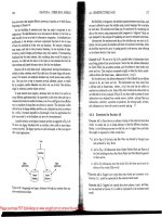
Consider the algebraic expression
Please purchase PDF Split-Merge on www.verypdf.com to remove this watermark.
CHAPTER
10.
LOGIC,4L QUERY LANGUAGES
tirle, year
O
length
>=
100
*
studioName
=
'
Fox1
Movie Movie
Figure
10.2: Expression tree
1.
W(t,y,l,c,s,p)
c
Movie(t,y,l,c,s,p)
AND

12
100
2. x(t,y,l,c,s,p)
t
Movie(t,y,l,c,s,p)
AND
s
=
'Fox'
3.
~(t,y,l,c,s,p)
t
W(t,y,l,c,s,p)
AND
X(t,y,l.c,s,p)
4.
Z(t,y)
+-
Y(t,y,l,c,s,p)
Figure 10.3: Datalog rules to perform several algebraic operations
from Example
5.10, whose expression tree appeared in Fig.
5.8.
We repeat
this tree
as
Fig. 10.2. There are four interior nodes, so we need to create four
IDB predicates. Each of these predicates
has a single Datalog rule, and we
summarize all the rules in Fig. 10.3.

The lowest two interior nodes perform simple selections on the
EDB
rela-
tion Movie, so we can create the
IDB
predicates
W
and
X
to represent these
selections. Rules
(1)
and (2) of Fig. 10.3 describe these selections. For example,
rule (1) defines
W
to be those tuples of Movie that have a length at least 100.
Then rule (3) defines predicate
Y
to be the intersection of
tY
and
X,
us-
ing the form of rule we learned for an intersection in Section 10.2.1. Finally,
rule (4) defines predicate
Z
to be the projection of
Y
onto the title and
.

year attributes. UTe here use the technique for simulating a projection that we
learned in Section 10.2.4. The predicate
Z
is the "answer" predicate; that is.
regardless of the value of relation Movie, the relation defined by
Z
is the same
as
the result of the algebraic expression with which we began this example.
Sote that, because
Y
is defined by a single rule, we can substitute for the
I;
subgoal in rule (4) of Fig. 10.3, replacing it with the body of rule (3). Then,
we can substitute for the
W
and
X
subgoals, using the bodies of rules (1) and
(2). Since the Movie subgoal appears in both of these bodies, we can eliminate
one copy. As a result,
Z
can be defined by the single rule:
Z(t,y)
t
Movie(t,y,l,c,s,p)
AND
1
2
100

AND
s
=
'Fox1
10.2.
FROM RELATIORrAL ALGEBRA TO DATALOG
479
Hon-ever, it is not common that a complex expression of relational algebra is
equivalent to a single
Datalog rule.
10.2.9
Exercises
for
Section
10.2
Exercise
10.2.1
:
Let R(a, b, c),
S(a,
6,
c), and T(a,
b,
c) be three relations.
Write one or more Datalog rules that define the result of each of the following
expressions of relational algebra:
a) R
U
S.
b)

R
n
S.
C) R-S.
*
d) (R
U
S)
-T.
!
e) (R- S)
n
(R-
T).
f) Za.b(R).
*!
g) ~a,b(R)
n
~"(n.6) (xb,e(S))-
Exercise
10.2.2
:
Let R(x, y, z) be a relation. Write one or more Datalog rules
that define
ac(R), where
C
stands for each of the following conditions:
a)
x=y.
*

b) x
<
y
AND
y
<
z.
c) x<yORy<z.
d)
NOT
(x
<
y
OR
.L.
>
y).
1
*!
e)
NOT
((x
<
y
OR
x
>
y)
AND
y

<
z)
1
!
f)
NOT
((x
<
y
ORx<
z)
AND
y <z).
Exercise
10.2.3
:
Let R(a.
b,
c),
S(b, c,
d),
and
T(d,
e) be three relations. Write
single Datalog rules for each of the natural joins:
a) R w
S.
b)
SwT.
c)

(R
w
S)
w
T.
(;Vote: since the natural join is associative and commuta-
tive. the order of the join of these three relations is irrelevant.)
Exercise
10.2.4
:
Let
R(x.
y, z) and S(x,
y,
z)
be two relations. Write one or
more
Datalog rules to define each of the theta-joins R
S,
where
C
is one
of the conditions of Exercise 10.2.2. For each of these conditions, interpret
each arithmetic comparison as comparing an attribute of
R
on the left with an
attribute of
S
on the right. For instance,
x

<
y
stands for R.x
<
S.Y.
Please purchase PDF Split-Merge on www.verypdf.com to remove this watermark.
480
CHAPTER
10.
LOGICAL QUERY LANGUAGES
!
Exercise
10.2.5:
It is also possible to convert Datalog rules into equivalent
relational-algebra expressions. While we have not discussed the method of doing
so in general, it is possible to work out many simple examples. For each of the
Datalog rules below, write an expression of relational algebra that defines the
same relation as the head of the rule.
*a)
P(x,y)
t
Q(x,z)
AND
R(z,y)
c) P(x,y)
t
Q(x,z)
AND
R(z,y)
AND

x
<
Y
10.3
Recursive Programming in Datalog
While relational algebra can express many useful operations on relations, there
are some computations that cannot be written as an expression of relational al-
gebra.
A
common kind of operation on data that we cannot express in relational
algebra involves an infinite, recursively defined sequence of similar expressions.
Example
10.22
:
Often, a successful movie is followed by a sequel; if the se-
quel does well, then the sequel has a sequel, and so on. Thus, a movie may
be ancestral to a long sequence of other movies. Suppose we have a relation
Sequelof (movie, sequel) containing pairs consisting of a movie and its iin-
mediate sequel. Examples of tuples in this relation are:
movie sequel
Naked
Gun
Naked
Gun
2112
Naked
Gun
2112
Naked
Gun

33113
We might also have a more general notion of a
follow-on
to a movie, which
is a sequel, a sequel of a sequel, and so on. In the relation above,
Naked
Gun
33113
is a follow-on to
Naked Gun,
but not a sequel in the strict sense we are
using the term "sequel" here. It saves space if we store only the immediate
sequels in the relation and construct the follow-ons if we need them. In the
above example, we store only one fewer pair, but for the five
Rocky
mories we
store six fewer pairs, and for the 18
Fkiday the 13th
movies we store 136 fewer
pairs.
Howeyer, it is not immediately obvious how we construct the relation of
follolv-ons from the relation SequelOf. We can construct the sequels of sequels
by joining SequelOf with itself once. An example of such an expression in
relational algebra, using renaming so that the join becomes a natural join, is:
-
In this expression, Sequelof is renamed twice, once so its attributes are called
first
and
second, and again so its attributes are called second and third.
10.3.

RECURSIVE PROGRAMhfING IN DATALOG
481
Thus, the natural join asks for tuples
(ml, m2)
and (ma, m4) in Sequelof such
that
mz
=
m3.
\iTe then produce the pair
(ml,
m4).
Note that m4 is the sequel
of the sequel of
ml.
Similarly, we could join three copies of Sequelof to get the sequels of sequels
of sequels
(e.g.,
Rocky
and
Rocky
IIq.
We could in fact produce the ith sequels
for any fixed value of
i
by joining Sequelof with itself
i
-
1
times. We could

then take the union of
Sequelof and a finite sequence of these joins to get all
the sequels up to some fixed limit.
What we cannot do in relational algebra is ask for the "infinite union" of the
infinite sequence of expressions that give the ith sequels for
i
=
1,2,.
. . .
Note
that relational algebra's union allows us only to take the union of
two relations;
not an infinite number. By applying the union operator any finite number of
times in an algebraic expression, we can take the union of any finite number of
relations. but we cannot take the union of an unlimited number of relations in
an algebraic expression.
10.3.1 Recursive Rules
By using an IDB predicate both in the head and the body of rules, we can
express an infinite union in
Datalog. We shall first see some examples of how
to express recursions in
Datalog. In Section 10.3.2 we shall examine the
least
fixedpoint
computation of the relations for the IDB predicates of these rules.
A
new approach to rule-evaluation is needed for recursive rules, since the straight-
forward rule-evaluation approach of Section 10.1.4 assumes all the predicates
in the body of rules have fixed relations.
Example

10.23:
We can define the IDB relation FollowOn by the following
tn-o Datalog rules:
1.
FollowOn(x, y)
t
SequelOf (x,y)
2.
FollowOn(x,
y)
t-
Sequelof (x,z)
AND
FollowOn(z, y)
The first rule is the basis: it tells us that every sequel is a follow-on. The second
rule says that every follow-on of a sequel of movie
x
is also a follo~v-on of
x.
More precisely: if
t
is a sequel of
x.
and we have found that
y
is a follow-on of
2.
then
y
is a folloir-on of

x.
10.3.2 Evaluating Recursive Datalog Rules
To
evaluate the IDB predicates of recursive Datalog rules.
we
follo\r the principle
that
we never want to conclude that a tuple is in an IDB relation unless
11-e
are
forced to do so by applying the rules as in Section
10.1.4. Thus. n-e:
1. Begin by assuming all IDB predicates have enipty relations.
2. Perform a number of
rounds:
in \vliich progressively larger relations are
constructed for the
IDB
predicates. In the bodies of the rules. use the
Please purchase PDF Split-Merge on www.verypdf.com to remove this watermark.
482
CHAPTER
10.
LOGICAL QUERY LANGUAGES
IDB relations constructed on the previous round. Apply the rules to get
new estimates for all the IDB predicates.
3.
If the rules are safe, no IDB tuple can have a component value that does
not also appear in some EDB relation. Thus, there are a finite number of
possible tuples for all IDB relations, and eventually there will be a round

on which no new tuples are added to any IDB relation. At this point,
we
can terminate our computation with the answer; no new IDB tuples mill
ever be constructed.
This set of IDB tuples is called the
least fiedpoint
of the rules.
Example
10.24
:
Let us show the computation of the least fixedpoint for
relation FollowOn when the relation SequelOf consists of the following three
tuples:
movie
I
sequel
At the first round of computation, FollowOn is assumed empty. Thus, rule
(2)
cannot yield any FollowOn tuples. However, rule (1) says that every SequelOf
tuple is a
FollowOn tuple. Thus, after the first round, the value of FollowOn is
identical to the
Sequelof relation above. The situation after round
1
is shown
in Fig. 10.4(a).
In the second round, we use the relation from Fig. 10.4(a) as FollowOn and
apply the two rules to this relation and the given
SequelOf relation. The first
rule gives us the three tuples that we already have, and in fact it is easy to see

that rule (1) will never yield any tuples for FollowOn other than these three.
For rule
(2), we look for a tuple from SequelOf whose second component equals
the first component of a tuple from FollowOn.
Thus, we can take the tuple
(Rocky,Rocky 11) from Sequelof and pair
it with the tuple (Rocky
11,Rocky 111) from FollowOn to get the new tuple
(Rocky, Rocky
111)
for FollouOn. Similarly, we can take the tuple
(Rocky
11, Rocky 111)
from SequelOf and tuple (~ocky II1,Rocky IV) from FollowOn to get new
tuple (Rocky 11,Rocky IV) for FollowOn. However, no other pairs of tuples
from SequelOf and
FollowOnjoin. Thus, after the second round, FollowOn has
the five tuples shown in Fig.
10 l(b). Intuitively, just
as
Fig. 10.4(a) contained
only those follow-on facts that are based on a single sequel, Fig.
10.4(b) contains
those follow-on facts based on one or two sequels.
In the third round, we use the relation from Fig. 10.4(b) for FollowOn and
again evaluate the body of rule (2).
\Ve
get all the tuples we already had.
of course, and one more tuple. When we join the tuple (Rocky,Rocky
11)

10.3.
RECURSIVE PROGRAIM~I~ING
IN
DilTALOG
(a) After round 1
Rocky Rocky
I1
Rocky
I1
Rocky
I11
Rocky
111
Rocky
IV
Rocky Rocky
I11
Rocky
I1
Rocky
IV
i
(b) After round
2
Rocky Rocky
I11
Rocky Rocky
IV
(c) After round
3

and subsequently
Figure 10.1: Recursive
conlputation of relation FollowOn
from SequelOf
with the tuple (Rocky 11,Rocky IV) fro111 the current value of
FollowOn,
we get the new tuple (Rocky, Rocky IV). Thus, after round
3,
the
value of FollowOn is as shown in Fig. 10.1(c).
When we proceed to round
4.
we get no new tuples, so we stop. The true
relation FollowOn is as shon-n in Fig.
10.4
(c).
There is an important trick that sinlplifies all recursire Datalog evaluations,
such as the
one above:
At any round, the only new tuples added to any IDB relation will come
from applications of rules in which at least one IDB
subgoal is matched
to a tuple that
was added to its relation at the previous round.
Please purchase PDF Split-Merge on www.verypdf.com to remove this watermark.
484
CHAPTER
10.
LOGICAL QUERY LANGUAGES
Other

Forms of Recursion
In Example 10.23 we used a
right-recursive
form for the recursion,
where the use of the recursive relation FollowOn appears after the EDB re-
lation SequelOf. We could
dso write similar
left-recursive
rules by putting
the recursive relation first. These rules are:
1.
FollowOn(x, y)
t
SequelOf (x, y)
2.
FollowOn(x, y)
t
FollowOn(x, z)
AND
SequelOf (z, y)
Informally,
y
is
a
follow-on of x if it is either a sequel of
x
or a sequel of a
follow-on of x.
We could even use the recursive relation twice,
as

in the
nonlinear
recursion:
1.
FollowOn(x, y)
t
SequelOf (x,y)
2.
FollowOn(x, y)
t
FollowOn (x
,
z)
AND
FollowOn (z
,
y)
Informally,
y
is a follow-on of
x
if it is either a sequel of
x
or a follow-on of
a follow-on of x. All three of
thtse forms give the same value for relation
FollowOn: the set of pairs (x,
y)
such that
y

is a sequel of a sequel of
.
.
.
(some number of times) of
x.
The justification for this rule is that should all subgoals be matched to "old"
tuples, the tuple of the head would already have been added on the previous
round. The next two examples illustrate this strategy and also show us more
complex examples of recursion.
Example
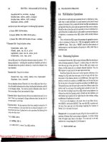
10.25:
Many examples of the use of recursion can be found in a
study of paths in
a
graph. Figure 10.5 shows a graph representing some flights of
two hypothetical airlines
-
Untried Airlines
(UA),
and
Arcane Airlines
(AA)
-
among the cities
San
Rancisco, Denver, Dallas, Chicago, and New York.
We may imagine that the flights are represented by an EDB relation:
Flights(airline, from, to, departs, arrives)
The tuples in this relation for the data of Fig. 10.5 are

shown in Fig. 10.6.
The simplest recursive question we can
ask
is "For what pairs of cities
(x,
y)
is it possible to get from city
x
to city
y
by taking one or more flights?" The
following two rules describe a relation Reaches
(x, y) that contains exactly these
pairs of cities.
1.
~eaches(x,y)
t
Flights(a,x,y,d,r)
2.
Reaches
(x,
y)
t
Reaches (x, z)
AND
Reaches (z
,
y)
10.3.
RECURSIVE PROGRALIbIING IN DATALOG

485
AA
1900-2200
Figure 10.5:
A
map of some airline flights
airline
U
A
A
A
U
A
U
A
A A
A A
A
A
U
A
from
SF
SF
DEN
DEN
D AL
D AL
CHI
CHI

to
-
-
DEN
D AL
CHI
DAL
CHI
NY
NY
NY
departs
930
900
1500
1400
1530
1500
1900
1830
arrives
1230
1430
1800
1700
1730
1930
2200
2130
Figure 10.6: Tuples in the relation Flights

The first rule says that Reaches contains those pairs of cities for which there
is a direct flight from the first to
the second; the airline
a,
departure time
d,
and arrival time
r
are arbitrary in this rule. The second rule says that if you
can reach from city
x
to city
r
and you can reach from
z
to
y,
then you can
reach
from
x
to
y.
Notice that we hare used the nonlinear form of recursion
here. as
~vas
described in the box on .'Other Forms of Recursion." This form is
slightly
more convenient here, because another use of Flights in the recursive
rule

~vould in\-olve three more variables for the unused components of Flights.
To evaluate the relation Reaches,
we follow the same iterative process intro-
duced in
Example 10.24. We begin by using Rule (1) to get the follo~ving pairs
in Reaches: (SF,
DEN).
(SF.
DAL). (DEN. CHI). (DEN. DAL). (DAL, CHI). (DAL, NY),
and
(CHI. NY).
These are the seven pairs represented by arcs in Fig. 10.5.
In
the nest round. we apply thr recursive Rule
(2)
to put together pairs
of arcs
such that the head of one
is
the tail of the next. That gives us the
additional pairs (SF:
CHI), (DEN, NY).
and (SF,
NY).
The third round combines
all one- and two-arc pairs together to form paths of length up to four arcs.
In this particular diagram, we get no new pairs. The relation Reaches thus
consists of the ten pairs
(x.
y)

such that
y
is reachable from
x
in the diagram
of Fig.
10.3. Because of the way we drew the diagram, these pairs happen to
Please purchase PDF Split-Merge on www.verypdf.com to remove this watermark.
CHAPTER
10.
LOGICAL QUERY LANGUAGES
be
exactly those (x,~) such that y is to the right of
z
in Fig 10.5.
Example
10.26:
A
more complicated definition of when two flights can be
combined into a longer sequence of flights is to require that the second leaves
an airport at least an hour after the first arrives at that airport. Now, we use
an
IDB
predicate, which we shall call
Connects(x,y,d,r),
that says we can
take one or more flights, starting at city x at time
d
and arriving at city y at
time

r.
If
there are any connections, then there is at least an hour to make the
connection.
The rules for
Connects
are:4
1.
Connects(x,y,d,r)
t
Flights(a,x,y,d,r)
2.
Connects(x,y,d,r)
t
Connects(x,z,d,tl) AND
Connects(z,y,t2,r) AND
tl
<=
t2
-
100
In the first round, rule (1) gives us the eight
Connects
facts shown above the
first line in Fig. 10.7 (the line is not part of the relation). Each corresponds
to one of the flights indicated in the diagram of Fig. 10.5; note that one of the
seven
arcs of that figure represents two flights at different times.
We now try to combine these tuples using Rule (2). For example, the second
and fifth of these tuples combine to give the tuple

(SF, CHI,
900,1730). However,
the second and sixth tuples do not combine because the arrival time in Dallas
is 1430, and the departure time from Dallas, 1500, is only half an hour later.
The
Connects
relation after the second round consists of all those tuples above
the first or second line in Fig.
10.7.
Above the top line are the original tuples
from round 1, and the six tuples added on round 2 are shown between the first
and second lines.
In the third round, we must in principle consider all pairs of tuples above
one of the
two lines in Fig. 10.7 as candidates for the two
Connects
tuples
in the body of rule (2). However, if both tuples are
above the first line, then
they would
have been considered during round
2
and therefore will not yield a
Connects
tuple we have not seen before. The only way to get a new tuple is if
at least one of the two
Connects
tuple used in the body of rule (2) were added
at the previous round;
i.e., it is between the lines in Fig. 10.7.

The third round
only gives us three new tuples. These are shown at the
bottom of Fig. 10.7. There are no new tuples in the fourth round, so our
computation is complete. Thus, the entire relation
Connects
is Fig. 10.7.
10.3.3
Negation in Recursive Rules
Sometimes it is necessary to use negation in rules that also involve recursion.
There is a safe
way
and an unsafe way to mix recursion and negation. Generally,
it
is considered appropriate to use negation only in situations where the negation
does not appear inside the fixedpoint operation. To see the difference, we shall
4~hese rules only work on the assumption that there are no connections spanning midnight.
F
f
g
10.3.
RECURSIVE PROGRAAfAfING IN DATALOG
b
x
-
-
SF
SF
DEN
DEN
DAL

D
AL
CHI
CHI
-
SF
SF
SF
DEN
DAL
DAL
-
SF
SF
SF
Y
-
DEN
DAL
CHI
D
AL
CHI
NY
NY
NY
-
CHI
CHI
D AL

Figure 10.7: Relation
Connects
after third round
consider
two
examples of recursion and negation, one appropriate and the other
paradoxical.
We shall see that only -'stratified" negation is useful when there
is recursion; the term .'stratified"
xvill be defined precisely after the examples.
Example
10.27
:
Suppose ~ve want to find those pairs of cities
(x,
y)
in the
map of Fig. 10.5 such that
U=l
flies from
x
to
y
(perhaps through several other
cities), but
AA
does not. 11-e can recursively define a predicate
UAreaches
as
we

defined
Reaches
in Example 10.25, but restricting ourselves only to
UX
flights,
as
follo~vs:
1.
UAreaches(x,y)
t
Flights(UA,x,y,d,r)
2.
are aches
(x, y)
t
are aches
(x,
Z)
AND UAreaches(z
,Y)
Similarly, rve can rccursively define the predicate
AAreaches
to be those pairs
of
cities
(r,
y)
such that one can travel fron~
x
to

y
using only
.I;\
flights, by:
1.
AAreaches(x,y)
+-
~lights(AA.x,~ *d*r)
2.
AAreaches
(x,
y)
t
reaches
(x,
2)
AND Atireaches
(z~Y)
Son-, it is a simple matter to compute the
UAonly
predicate consisting of those
pairs of cities
(x,
y) such that one can get from
x
to
y
on
UX
flights but not on

-\.A
flights, with the nonrecursive rule:
UAonly (x, y)
t
U~reaches(x, y) AND NOT ~~reaches(x,
y)
Please purchase PDF Split-Merge on www.verypdf.com to remove this watermark.
488 CHAPTER
10.
LOGlCAL QUERY LANGU-AGES
This rule computes the set difference of UAreaches and AAreaches.
For the data of Fig. 10.5, UAreaches is seen to consist of the
following pairs:
(SF, DEN), (SF, DAL), (SF, CHI), (SF, NY), (DEN,
DAL), (DEN, CHI), (DEN, NY), and
(CHI, NY). This set is computed by the iterative fixedpoint process outlined
in Section 10.3.2. Similarly, we can compute the value of AAreaches for this
data; it is: (SF, DAL), (SF, CHI), (SF, NY), (DAL, CHI), (DAL, NY), and
(CHI,
NY).
When
we take the difference of these sets of pairs we get: (SF, DEN), (DEN, DAL),
(DEN, CHI), and (DEN, NY). This set of four pairs is the relation UAonly.
Example
10.28
:
Now, let us consider an abstract example where things don't
work
as
well.

Suppose we have a single EDB predicate
R.
This predicate
is unary (one-argument), and it has a single tuple, (0). There are
two IDB
predicates,
P
and Q, also unary. They are defined by the two rules
1.
P(x)
t
R(x)
AND
NOT
Q(x)
2.
Q(x)
t
R(x)
AND
NOT
P(x)
Informally, the two rules tell us that an element
x
in
R
is either in
P
or in
Q

but not both. Sotice that
P
and Q are defined recursively in terms of each
other.
When we defined what recursive rules meant in Section 10.3.2. we said
we
want the least fixedpoint, that is, the smallest IDB relations that contain all
tuples that the rules require us to allow. Rule
(I), since it is the only rule for
P, says that as relations,
P
=
R-
Q,
and rule
(2)
likewise says that Q
=
R-P.
Since
R
contains only the tuple (0), we know that only (0) can be in either
P
or Q. But where is (0)? It cannot be in neither, since then the equations are
not satisfied; for instance
P
=
R
-
Q

would imply that 0
=
((0))
-
0, which is
false.
If
we let
P
=
((0)) while Q
=
0, then we do get a solution to both equations.
P
=
R
-
Q
becomes ((0))
=
((0))
-
0, which is true, and
Q
=
R
-
P
becomes
0

=
((0))
-
{(O)}, which is also true.
Hen-ever,
we can also let
P
=
0
and
Q
=
((0)). This choice too satisfies
both rules.
n'e thus have two solutions:
Both are minimal. in the
sense that if we throw any tuple out of any relation.
the resulting relations no longer satisfy the rules.
We cannot. therefore, decide
bet~veen the two least fisedpoints (a) and
(b).
so we cannot answer a si~nple
question such as -1s P(0) true?"
0
In Example 10.28,
we
saw that our idea of defining the meaning of recur-
sire rules by finding the least fixedpoint no longer works when recursio~i and
negation are tangled up too intimately.
There can be more than one least

fixedpoint, and these fixedpoints can contradict each other. It would be good if
-
some other approach to defining the meaning of recursive negation would work
10.3.
RECURSlIrE PROGRA&IAlING
IN
DATALOG
489
better, but unfortunately, there is no general agreement about what such rules
should mean.
Thus, it is conventional to restrict ourselves to recursions in which nega-
tion is
stratified.
For instance, the SQL-99 standard for recursion discussed in
Section 10.4 makes this restriction.
As
we shall see, when negation is stratified
there is an algorithm to compute one particular least fixedpoint (perhaps out of
many such fixedpoints) that matches our intuition about what the rules mean.
We define the property of being stratified
as
follows.
1.
Draw a graph whose nodes correspond to the IDB predicates.
2. Draw an arc from node
'4
to node
B
if a rule with predicate
A

in the head
has
a
negated subgoal with predicate
B.
Label this arc with
a
-
sign to
indicate it is a
negative
arc.
3. Draw an arc from node
A
to node
B
if a rule with head predicate
A
has a non-negated subgoal with predicate
B.
This arc does not have
a
minus-sign as label.
If this graph
has
a cycle containing one or more negative arcs, then the
recursion is not stratified. Otherwise, the recursion is stratified. We can group
the IDB predicates of a stratified graph into
strata.
The stratum of a predicate

I
is the la~gest number of negative arcs on a path beginning from
A.
If the recursion is stratified. then we may evaluate the IDB predicates in
the order of their strata,
lolvest first. This strategy produces one of the least
fixedpoints of the rules.
1Iore importantly, cornputi~lg the IDB predicates in
the order
implied by their strata appears always to make sense and give us the
.'rights fixedpoint. I11 contrast, as we have seen in Example 10.28, unstratified
recursions
may leave us with no .'rightv fixedpoint at all, even if there are many
to choose
from.
UAonly
AAreaches
UAreaches
Figure 10.8: Graph constructed from a stratified recursion
Example
10.29
:
The graph for the predicates of Example 10.27 is shown in
Fig.
10.8. AAreaches and UAreaches are in stratum 0: because none of the
paths beginning at their nodes involves a
negative arc. UAonly has stratum 1,
because there are paths
with one negative arc leading from that node, but no
paths with more than one negative arc. Thus,

we must completely evaluate
AAreaches and UAreaches before we start evaluating UAonly.
Please purchase PDF Split-Merge on www.verypdf.com to remove this watermark.
490
CHAPTER
10.
LOGICAL
QUERY
LANGUAGES
Compare the situation when we construct the graph for the IDB predicates
of Example 10.28. This graph is shown in Fig. 10.9. Since rule
(1)
has head
P
with negated subgoal
Q,
there is a negative arc from
P
to
Q.
Since rule
(2)
has head
Q
with negated subgoal
P,
there is also a negative
arc
in the opposite
direction. There is thus a negative cycle, and the rules are not stratified.

Figure 10.9: Graph constructed from an unstratified recursion
10.3.4
Exercises
for
Section
10.3
Exercise
10.3.1
:
If we add or delete arcs to the 'diagram of Fig. 10.5, we
may change the value of the relation Reaches of Example 10.25, the relation
Connects of Example 10.26, or the relations
UAreaches and AAreaches of Ex-
ample 10.27. Give the new
values of these relations if we:
*
a) Add an arc from
CHI
to SF labeled
AA,
1900-2100.
b)
4dd an arc from
NY
to
DEN
labeled
UA,
900-1100.
c)

.4dd both arcs from (a) and (b).
d) Delete the arc from
DEN
to
DAL.
Exercise
10.3.2
:
Write Datalog rules (using stratified negation, if negation
is necessary) to describe the following modifications to the notion of
"follolv-
on" from Example 10.22. You may use
EDB
relation Sequelof and the IDB
relation
FollowOn defined in Example 10.23.
*
a) P(x,
y)
meaning t.hat movie
y
is a follow-on to movie
x,
but not a sequel
of
z
(as
defined by the
EDB
relation Sequelof).

b)
Q(x,
y) meaning that
y
is a follow-on of
x,
but neither a sequel nor a
sequel of a sequel.
!
cj R(x) meaning that movie
x
has at least two follow-ons. Mote that both
could be sequels, rather than one being a sequel and the other a sequel of
a
sequel.
!!
d)
S (x,
y
1,
meaning that
y
is
a follow-on of
x
but
y
has at most one follow-on.
10.3.
RECURSIVE PROGRAbIhIING IN DATALOG

491
Exercise
10.3.3:
ODL classes and their relationships can be described by
a relation
Rel(class, rclass, mult). Here, mult gives the multiplicity of
a relationship, either
multi for a multivalued relationship, or single for a
single-valued relationship. The first
two attributes are the related classes; the
relationship goes from class to
rclass (related class). For example, the re-
lation
Re1 representing the three
ODL
classes of our running movie example
from Fig.
4.3
is show11 in Fig. 10.10.
class
(
rclass
1
mult
Star
1
Movie
1
multi
Movie Star

1
mlti
Movie Studio single
Studio Movie multi
Figure 10.10: Representing ODL relationships by relational data
\Ye can also see this data as a graph, in which the nodes are classes and
the arcs go from a class to a related class,
with label multi or single,
as
appropriate. Figure 10.11 illustrates this graph for the data of Fig. 10.10.
multi
single
7-
Star Movie Studio
/' '
multi rnulti
Figure 10.11: Representing relationships by
a
graph
For each of the following, write
Datalog rules, using stratified negation if
negation is necessary, to express the described
predicate(s). You may use Re1
as
an
EDB
relation. Show the result of evaluating your rules: round-by-round,
on the data from
Fig.
10.10.

a) Predicate
P(class, eclass)
,
meaning that there is
a
path5 in the graph
of classes that goes from class to
eclass. The latter class can be thought
of
as
"embedded" in class, since it is in a sense part of a part of an
-
. .
ob-
ject of the first class.
*!
b) Predicates S(class, eclass) and M(class, eclass). The first means
that there is a .'single-valued embedding" of eclass in class. that is, a
path
from class to eclass along 1%-liich every arc is labeled single. The
second.
Jf.
lizeans that there is a .'multivalued embedding" of eclass in
class. i.e a path from class to eclass with at least one arc labeled
multi.
'We shall not consider empty paths to be "paths" in this exercise.
Please purchase PDF Split-Merge on www.verypdf.com to remove this watermark.
492
CH.4PTER
10.

LOGICAL QUERY LANGUAGES
c) Predicate
Q(class, eclass)
that says there is a path from
class
to
eclass
but no single-valued path. You may use IDB predicates defined
previously in this exercise.
10.4
Recursion
in
SQL
The SQL-99 standard includes provision for recursive rules, based on the recur-
sive
Datalog described in Section 10.3. Although this feature is not part of the
"coren SQL-99 standard that every
DBMS
is expected to implement, at least
one major system
-
IBM's DB2
-
does implement the SQL-99 proposal. This
proposal differs from our description in two ways:
1.
Only
linear
recursion, that
is,

rules with at most one recursive subgoal, is
mandatory. In what follows, we shall ignore this restriction; you should
remember that there could be
an
implementation of standard SQL that
prohibits nonlinear recursion but allows linear recursion.
2. The requirement of stratification, which we discussed for the negation
operator in Section 10.3.3, applies also to other operators of SQL that
can cause similar problems, such
as
aggregations.
10.4.1
Defining
IDB
Relations
in
SQL
The
WITH
statement allows us to define the SQL equivalent of IDB relations.
These definitions can then be used within the
WITH
statement itself.
X
simple
form of the
WITH
statement is:
WITH
R

AS
<definition of R> <query involving R>
That is, one defines a temporary relation named R, and then uses R in some
query. More generally, one can define several relations after the
WITH,
separating
their definitions by commas. Any of these definitions may be recursive. Sev-
eral defined relations may be mutually recursive; that is, each may be defined
in terms of some of the other relations, optionally including itself. However,
any relation that is involved in a recursion must be preceded by the keyword
NZCURSIVE.
Thus, a
WITH
statement has the form:
1.
The keyword
WITH.
2.
One or more definitions. Definitions are separated by commas, and each
definition consists of
(a)
An optional keyword
RECURSIVE,
which is required if the relation
being defined is recursive.
(b)
The name of the relation being defined.
(c)
The keyword
AS.

10.4.
RECURSION IN SQL
(d) The query that defines the relation.
3.
h
query, which may refer to any of the prior definitions, and forms the
result of the
WITH
statement.
It is important to note that, unlike other definitions of relations, the def-
initions inside a
WITH
statement are only available within that statement and
cannot be used elsewhere. If one wants a persistent relation, one should define
that relation in the database schema, outside any
WITH
statement.
Example
10.30
:
Let us reconsider the airline flights information that we used
as
an example in Section 10.3. The data about flights is in a relationB
Flights (airline, f rm, to, departs
arrives)
The actual data for our example
was
given in Fig. 10.5.
In Example
10.25, we computed the

IDB
relation
Reaches
to be the pairs of
cities such that it is possible to fly from the first to the second using the flights
represented by the
EDB
relation
Flights.
The two rules for
Reaches
are:
1.
Reaches(x,y)
t
~lights(a,x,~,d,r)
2.
Reaches
(x,
y)
t
~eaches
(X
,z)
AND
Reaches
(2,~)
From these rules, we can develop an SQL query that produces the relation
Reaches.
This SQL query places the rules for

Reaches
in a
WITH
statement,
and follows it by a query. In Example 10.25, the desired result
\\-as the entire
Reaches
relation. but we could also ask some query about
Reaches.
for instance
the set of cities reachable
from Denver.
1)
WITH RECURSIVE
~eaches
(f
rm, to)
AS
2)
(SELECT
frm, to FROM
lights)
3)
UNION
4)
(SELECT
Rl.frm, R2.to
5)
FROM Reaches R1, Reaches R2
6)

WHERE
Rl.to
=
R2.frm)
7)
SELECT
*
FROM Reaches;
Figure 10.12: Recursive SQL query for pairs of reachable cities
Figure 10.12
slio~\-s lion to compute
Reaches
as an SQL quer?. Line
(1)
introduces the definition of
Reaches,
while the actual definition of this relation
is in lines (2) through
(6).
That definition is a union of two queries, corresponding to the two rules
by
which
Reaches
was defined in Example 10.25. Line
(2)
is the first term
6\\'e changed the name
of
the second attribute
to

frm,
since
from
in
SQL
is
a
ke~lvord.
Please purchase PDF Split-Merge on www.verypdf.com to remove this watermark.
494
CHAPTER
10.
LOGICAL QUERY LAhiGUA4GES
Mutual Recursion
There is a graph-theoretic way to check whether two relations or predi-
cates are mutually recursive. Construct a
dependency
graph whose nodes
correspond to the relations (or predicates if we are using
Datalog rules).
Draw an arc from relation
A
to relation
B
if the definition of B depends
directly on the definition of
A.
That is, if Datalog is being used, then
-4
appears in the body of a rule with B at the head. In SQL,

A
would appear
somewhere in the definition of B, normally in a
FROM
clause, but possibly
as
a
term in a union, intersection, or difference.
If
there is
a
cycle involving nodes
R
and
S,
then
R
and
S
are
mutually
recursive.
The most common case will be
a
loop from
R
to
R,
indicating
that

R
depends recursively upon itself.
Note that the dependency graph is similar to the graph we introduced
,
in Section 10.3.3 to define stratified negation. However, there we had to
1
distinguish between positive and negative dependence, while here we do
/
not make that distinction.
of the union and corresponds to the first, or basis rule. It says that for every
tuple in the
Flights
relation, the second and third components (the
frm
and
to
components) are
a
tuple in
Reaches.
Lines (4) through
(6)
correspond to the second, or inductive, rule in the
definition of
Reaches.
The tm-o
Reaches
subgoals are represented in the
FROM
clause by two aliases

R1
and
R2
for
Reaches.
The first component of
R1
cor-
responds to
.2:
in Rule (2), and the second component of
R2
corresponds to
y.
\-ariable
z
is represented by both the second component of
R1
and the first
component of
R2;
note that these components are equated in line
(6).
Finally, line
(7)
describes the relation produced by the entire query. It is
a
copy of the
Reaches
relation. As an alternative, we could replace line

(7)
by a
more complex query. For instance,
7)
SELECT to FROM Reaches WHERE frm
=
'DEN';
~vould produce all those cities reachable from Denver.
10.4.2
Stratified Negation
The queries that can appear as the definition of a recursive relation are not
arbitrary SQL queries. Rather, they must be restricted in certain ways: one of
the most important requirements is that negation of
niutually recursive relations
be stratified, as discussed in Section 10.3.3. In Section 10.4.3, we shall see hoa
the principle of stratification extends to other constructs that we find in SQL
but not in Datalog, such as aggregation.
10.4.
RECURSION IN
SQL
Example
10.31
:
Let us re-examine Example 10.27, where we asked for those
pairs of cities
(x,
y)
such that it is possible to travel from
x
to

y
on the airline
UA,
but not on
XA.
1%
need recursion to express the idea of traveling on one
airline through an indefinite sequence of hops. However, the negation aspect
appears in a stratified
way: after using recursion to compute the two relations
UAreaches
and
AAreaches
in Example 10.27, we took their difference.
We could adopt the same strategy to write the query in SQL. However,
to illustrate a different way of proceeding, we shall instead define recursively a
single relation
Reaches (airline, f
nu,
to),
whose triples
(a,
f,
t)
mean that one
can fly
from city
f
to city
t,

perhaps using several hops but using only flights of
airline
a.
Ifre shall also use a nonrecursive relation
Triples (airline, f rm, to)
that is the projection of
Flights
onto the three relevant components. The
query is shown in Fig. 10.13.
The definition of relation
Reaches
in lines (3) through
(9)
is the union of
two terms. The basis term is the relation
Triples
at line
(4).
The inductive
term is the query of lines
(6)
through (9) that produces the join of
Triples
with
Reaches
itself. The effect of these two terms is to put into
Reaches
all
tuples (a,
f,

t)
such that one can travel from city
f
to city
t
using one or more
hops, but
with all hops on airline
a.
The query itself appears in lines (10) through (12). Line (10) gives the city
pairs reachable via
U.4,
and line (12) gives the city pairs reachable via
A.4.
The
result of the query is the difference of these two relations.
1) WITH
2)
Triples AS SELECT airline, frm, to FROM Flights,
3)
RECURSIVE Reaches(airline, frm, to) AS
4)
(SELECT
*
FROM ~riples)
5)
UNION
6)
(SELECT Triples.airline, Triples.frm, Reachhs.to
7

FROM Triples, Reaches
8
WHERE Triples.to
=
Reaches.frm AND
9
>
Triples.airline
=
Reaches.airline)
10)
(SELECT'frm, to FROM Reaches WHERE airline
=
'UA')
11) EXCEPT
12)
(SELECT frm, to FROM Reaches WHERE airline
=
'AA');
Figure 10.13: Stratified query for cities reachable by one of tn-o airlines
Example
10.32
:
In Fig. 10.13, the negation represented by
EXCEPT
in line (11)
is clearly stratified, since it applies only after the recursion of lines (3) through
Please purchase PDF Split-Merge on www.verypdf.com to remove this watermark.
496
CHAPTER

10.
LOGICAL QUERY LANGUAGES
(9) has been completed. On the other hand, the use of negation in Exam-
ple 10.28, which we observed was unstratified, must be translated into a use of
EXCEPT
within the definition of mutually recursive relations. The straightfor-
ward translation of that example into SQL is shown in Fig.
10.14. This query
asks
only for the value of
P,
although we could have asked for Q, or some
function of
P
and Q.
1)
WITH
2)
RECURSIVE P(x) AS
3)
(SELECT
*
FROM R)
4)
EXCEPT
5)
(SELECT
*
FROM
Q),

6)
RECURSIVE Q(x) AS
7)
(SELECT
*
FROM R)
8
EXCEPT
9
>
(SELECT
*
FROM P)
10) SELECT
*
FROM P;
Figure 10.14: Unstratified query, illegal in SQL
The two uses of
EXCEPT,
in lines (4) and
(8)
of Fig. 10.14 are illegal in SQL,
since in each case the second argument is a relation that is mutually recursive
with the relation being defined. Thus, these uses of negation are not stratified
negation and therefore not permitted. In fact, there is no work-around for this
problem in SQL, nor should there be, since the recursion of Fig. 10.14 does not
define unique values for relations
P
and
Q.

10.4.3
Problematic Expressions in Recursive
SQL
\Ye have seen in Example 10.32 that the use of
EXCEPT
to help define a recursive
relation can violate
SQL's requirement that negation be stratified. Hon-ever,
there are other unacceptable forms of query that do not use
EXCEPT.
For in-
stance, negation of a relation can also be expressed by the use of
NOT IN.
Thus.
lines (2) through (5) of Fig. 10.14 could also have been written
RECURSIVE P(x) AS
SELECT x FROM R WHERE x NOT IN
Q
This
rewriting still leaves the recursion unstratified and therefore illegal.
On the other hand, simply using
NOT
in a
WHERE
clause, such
as
NOT x=y
(which could be written
xoy
anyway) does not automatically violate the con-

dition
that
negation be stratified. What then is the general rule about what
sorts of
SQL queries can be used to define recursive relations in SQL?
10.4.
RECURSION
IN
SQL
497
The principle is that to be a legal SQL recursion, the definition of a recursive
relation R may only involve the use of a mutually recursive relation
S
(S
can
-
-
be
R
itself) if that use is
monotone
in
S.
d
use of
S
is monotone if adding an
arbitrary tuple to
S
might add one or more tuples to R, or it might leave R

unchanged, but it can never cause any tuple to be deleted from R.
This rule
makes sense when one considers the least-fixedpoint computation
outlined in Section 10.3.2.
\Ire start with our recursively defined IDB relations
empty, and
we repeatedly add tuples to them in successive rounds. If adding
a tuple in one round could cause us to have to delete a tuple at the next
round, then there is the risk of oscillation, and the fixedpoint computation
might never converge. In the following examples, we shall see some constructs
that are nonmonotone and therefore are
outlawed in SQL recursion.
Example 10.33
:
Figure 10.14 is an implementation of the Datalog rules for
the unstratified negation of Example 10
28.
There, the rules allo~ved two differ-
ent minimal fixedpoints.
As expected, the definitions of
P
and Q in Fig. 10.14
are not monotone. Look at the definition of
P
in lines (2) through (5) for in-
stance.
P
depends on Q. with which it is mutually recursive, but adding a tuple
to
Q

can delete a tuple from
P.
To see why, suppose that
R
consists of the two
tuples (a) and (b), and
Q
consists of the tuples (a) and
(c).
Then
P
=
{(b)).
Holvever, if lve add (b) to Q, then
P
becomes empty. Addition of a tuple to Q
has caused the deletion of a tuple from
P,
so
we
have a nonmonotone, illegal
construct.
This lack of monotonicity leads directly to an oscillating behavior when we
try to evaluate the relations
P
and
Q
by computing
a
minimal fi~ed~oint.~ For

instance, suppose that
R
has the two tuples {(a),
(b)).
Initially. both
P
and Q
are empty. Thus. in the first round. lines (3) through (5) of Fig. 10.14 compute
P
to have value {(a), (b)). Lines
(7)
through (9) compute
Q
to have the same
value, since the old. empty value of
P
is used at line (9).
Sow, both
R,
P,
and Q have the value {(a), (b)}. Thus, on the next tound,
P
and
Q
are each computed to be empty at lines (3) through (5) and
(7)
through (9). respectively. On the third round, both would therefore get the
value {(a), (b)). This process continues forever,
with both relations empty on
el-en rounds and {(a), (b)) on odd rounds. Therefore, we never obtain clear

values for the
two relations
P
and
Q
from their "definitions" in Fig. 10.14.
I
Example 10.34
:
-1ggregation can also lead to nonmonotonicity, although the
connection
may not be obvious at first. Suppose lye have unary (one-attribute)
relations
P
and
Q
defined by the following two conditions:
1.
P
is the union of
Q
and an EDB relation
R.
'IVhen the recursion is not monotone. then the order in which we exaluate the relations in
a
WITH
clause can affect the final answer, although when the recursion is monotone, the result
is independent of order. In this and the next example,
we shall assume that on each round,
P

and
Q
are evaluated '-in parallel." That is. the old value of each relation is used to compute
the other at each round. See the box on
'.Using Kew Values in Fixedpoint Calculations."
Please purchase PDF Split-Merge on www.verypdf.com to remove this watermark.
498
CHAPTER
10.
LOGICAL QUERY
LANGUAGES
2.
Q
has one tuple that is the sum of the members of
P.
We can express these conditions by a
WITH
statement, although this statement
violates the monotonicity requirement of SQL. The query shown in Fig. 10.15
asks for the value of
P.
1)
WITH
2)
RECURSIVE
P(x)
AS
3)
(SELECT
*

FROM R)
4)
UNION
5)
(SELECT
*
FROM Q)
,
6
1
RECURSIVE Q(x) AS
7)
SELECT SUM(x) FROM
P
8)
SELECT
*
FROM
P;
Figure 10.15: Nonrnonotone query involving aggregation, illegal in SQL
Suppose that
R
consists of the tuples (12) and (34), and initially
P
and
Q
are both empty, as they must be at the beginning of the fixedpoint computation.
Figure 10.16 summarizes the values computed in the first six rounds. Recall
that we have adopted the strategy that all relations are computed in one round
from the values at

the previous round. Thus,
P
is computed in the first round
to be the same
as
R,
and
Q
is empty, since the old, empty value of
P
is used
in line (7).
At the second round, the union of lines (3) through
(3)
is the set
R
=
{(12), (34)), so that becomes the new value of
P.
The old jalue of
P
was
the
same
as
the new value, so on the second round
Q
=
((46)). That is, 46 is the
sum of 12 and 34.

.At the third round, we get
P
=
{(12), (34), (46)) at lines (2) through
(5).
Using the old value of
P,
{(12), (34)),
Q
is defined by lines (6) and (7) to be
Figure 10.16: Iterative calculation of fixedpoint for a nonmonotone aggregation
10.4.
RECURSION
IAr
SQL
Using
New
Values
in
Fixedpoint Calculations
One might wonder why we used the old values of
P
to compute
Q
in
Esamples 10.33 and 10.34, rather than the new values of
P.
If
these
queries

n-ere legal, and we used new values in each round, then the query
results
might depend on the order in which n-e listed the definitions of the
recursive predicates in the
WITH
clause. In Example 10.33,
P
and
Q
n-ould
converge to one of the two possible fixedpoints, depending
011
the order of
evaluation. In Example 10.34,
P
and
Q
would still not converge, and in
fact they
would change at every round, rather than every other round.
((46)) again.
At
the fourth round,
P
has the same value, {(12), (34),(46)), but
Q
gets
the value
((92)): since 12+34+46=92. Notice that
Q

has lost the tuple (46),
although it gained the tuple
(92).
That is, adding the tuple (46) to
P
has
caused a tuple (by coincidence the same tuple) to be deleted from
Q.
That
behavior is the nonmonotonicity that SQL prohibits in recursive definitions,
confirming that the query of Fig. 10.15 is illegal. In general, at the
2ith round,
P
will consist of the tuples (12), (34, and
(46i
-
46), TI-hile
Q
consists only of
the tuple
(4%).
10.4.4
Exercises
for
Section
10.4
Exercise
10.4.1
:
In Example 10.23 we discussed a relation

Sequelof
(movie,
sequel)
that gil-FS the immediate sequels of a movie. \Ye also defined an
IDB
relation
FollowOn
whose pairs
(x.
y)
were movies such that
y
u-as either a sequel of
x,
a sequel of
a
sequel. or so on.
a)
Write the definition of
FollouOn
as an SQL recursion.
b)
Write a recursive SQL query that returns the set of pairs
(s,
y)
such that
movie
y
is a follo~v-on to movie
x.

but not a sequel of x.
c)
Ifiite a recursil-e SQL query that returns the set of pairs
(x.
y)
meaning
that
y
is
a
follo\v-on of
s,
but neither a sequel nor
a
sequel of a sequel.
!
d)
\Trite a recursil-e
SQL
query that returns the set of movies
.r
that have
at least
two follo~v-ons. Sote that both could be sequels. rather thau one
being a sequel and the other
a
sequel of a sequel.
!
e) Write a recursire SQL query that returns the set of pairs (x.
y)

such that
nlovie
y
is a follo~r-on of
z
but
y
has at most one follow-on.
Please purchase PDF Split-Merge on www.verypdf.com to remove this watermark.
500
CHAPTER
10.
LOGICAL QUERY LANGUAGES
Exercise
10.4.2
:
In Exercise
10.3.3,
we introduced a relation
that describes how one ODL class is related to other classes. Specifically, this
relation has tuple (c,
d,
m)
if there is a relation from class c to class
d.
This
relation is multivalued if m
=
'multi
'

and it is single-valued if
m
=
'
single
'
.
We
also
suggested in Exercise
10.3.3
that it is possible to view Re1 as defining
a
graph ~vhose nodes are classes and in which there is an arc from
c
to
d
labeled
rn
if
and
only if (c, d, m) is
a
tuple of Rel. Write
a
recursive SQL query that
produces the set of pairs (c,
d)
such that:
a) There is a path from class

c
to class
d
in the graph described above.
*
b)
There is
a
path from
c
to
d
along mhich every arc is labeled single.
*!
c) There is a path from c to d along which at least one arc is labeled rnulti.
d) There is a path from c to
d
but no path along which ail arcs are labeled
single.
!
e) There is
a
path from
c
to
d
along which arc labels alternate single and
multi.
f) There are paths from c to
d

and from d to c along which every arc is
labeled
single.
10.5 Summary of Chapter 10
+
Datalog: This form of logic allows us to write queries in the relational
model. In
Datalog, one n-rites rules in which a head predicate or relation
is defined in terms of a body. consisting of subgoals.
+
Atoms: The head and subgoals are each atoms, and an atom consists of
an (optionally negated) predicate applied to some number of arguments.
Predicates
may represent relations or arithmetic comparisons such as
<.
+
IDB
and
EDB
Predicates: Some predicates correspond to stored relations.
and
are ralled
EDB
(extensional database) predicates or relations. Other
prcdicatrs, called IDB (intensional database), are defined by the rules.
EDB predicates may not appear in rule heads.
+
Safe Rules: \fie generally restrict Datalog rules to be safe, meaning that
every variable in the rule appears in some nonnegated, relational
subgoal

of the body. Safe rules guarantee that if the EDB relations are finite, then
the IDB relations will be finite.
10.6.
REFEREATCES FOR CHAPTER
10
50
1
4
Relational Algebra and Datalog: All queries that can be expressed in
relational algebra can also be expressed in
Datalog. If the rules are safe
and nonrecursive, then they define exactly the same set of queries as
relational algebra.
4
Recursive Datalog: Datalog rules can be recursive, allowing
a
relation
to be defined in terms of itself. The meaning of recursive
Datalog rules
without negation is the least fixedpoint: the smallest set of tuples for the
IDB relations that makes the heads of the rules exactly equal to what
their bodies collectively imply.
fi
+
Stratified Negation: When a recursion involves negation, the least fixed-
$
point may not be unique, and in some cases there is no acceptable meaning

to the Datalog rules. Therefore, uses of negation inside a recursion must
$

be forbidden, leading to a requirement for stratified negation. For rules
8
of this type, there is one (of perhaps several) least fixedpoint that is the
generally accepted meaning of the rules.
+
SQL
Recursive Queries: In SQL, one can define temporary relations to be
used in a manner similar to IDB relations in
Datalog. These temporary
relations may be used to construct answers to queries recursively.
4
Stratification in SQL: Yegations and aggregations involved in an SQL re-
cursion
iliust be monotone, a generalization of the requirement for strat-
ified negation in
Datalog. Intuitively, a relation may not be defined,
directly or indirectly. in
terms of a negation or aggregation of itself.
1
10.6 References for Chapter 10
Codd introduced a form of first-order logic called relational calculus in one of
his early papers on the relational model
[4].
Relational calculus is an espression
language. much like relational algebra, and is in fact equivalent in expressive
pomer to relational algebra, a fact proved in
[4].
Datalog. looking more like logical rules, was inspired by the programming
language
Prolog. Because it allows recursion, it is more expressive than rela-

tional calculus. The book
[GI
originated much of the de\-elopn~ent of logic
as
a
query language.
~vhile
[2]
placed the ideas in the context of database systems.
The idea
that the stratified approach gives the correct choice of fixedpoint
comes from
[3].
although using this approach to evaluating Datalog rules xvas
the independent idea of
[I].
[8].
and
[lo].
Nore on stratified negation. on the
relationship
betxeen relational algebra, Datalog, and relational calculus; and
on the
e~aluation of Datalog rules: lvith or without negation. can be found
in
PI.
[7]
surveys logic-based query languages. The source of the
SQL-99
proposal

for recursion is
[j].
Please purchase PDF Split-Merge on www.verypdf.com to remove this watermark.
502
CHAPTER
10.
LOGICAL QUERY LANGUAGES
1.
Apt, K. R.,
H.
Blair, and
A.
Walker, "Towards a theory of declarative
knowledge," in
Foundations of Deductive Databases and Logic Program-
ming
(J. Minker,
ed.),
pp. 89-148, Morgan-Icaufmann, San Francisco,
1988.
2. Bancilhon,
F.
and R. Ramakrishnan, "An amateur's introduction to re-
cursive query-processing strategies,"
ACM
SZGMOD Intl. Conf. on Man-
agement of Data,
pp. 16-52, 1986.
3. Chandra,
A.

K. and D. Harel, "Structure and complexity of relational
queries,"
J.
Computer and System Sciences
25:l (1982), pp. 99-128.
4. Codd,
E.
F.,
"Relational completeness of database sublanguages," in
Database Systems
(R. Rustin, ed.), Prentice Hall, Engelwood Cliffs. iVJ,
1972.
5. Finkelstein, S. J.,
N.
Mattos, I. S. klumick, and
H.
Pirahesh, "Expressing
recursive queries in SQL,"
IS0 WG3 report X3H2-96-075, March, 1996.
6. Gallaire,
H.
and J. Minker,
Logic and Databases,
Plenum Press, New 'I'ork:
1978.
7.
M.
Liu; "Deductive database languages: problems and solutions,"
Com-
puting Surveys

31:l (March, 1999), pp. 27-62.
8. Naqvi, S.; "Negation as failure for first-order queries,"
Proc. Fifth
ACA4
Symp.
on
Principles of Database Systems,
pp. 114-122, 1986.
9.
Ullman, J. D.,
Principles of Database and Knowledge-Base Systems, Vol-
ume
I,
Computer Science Press, New York, 1988.
10. Van Gelder,
A.,
.'Negation as failure using tight derivations for general
logic programs," in
Foundations of Deductive Databases and Logic Pro-
gramming
(J. Minker, ed.), pp. 149-176, Morgan-Kaufmann, San Fran-
cisco: 1988.
Chapter
Data
Storage
This chapter begins our study of implementation of database management sys-
tems. The first issues we must address involve
how a DBMS deals with very
large
amounts of data efficiently. The study can be divided into txvo parts:

1.
How does a computer system store and manage very large amounts of
data?
2.
What representations and data structures best support efficient manipu-
lations of this data?
We cover (1) in this chapter and (2) in Chapters 12 through 14.
This chapter explains the devices used to store massive amounts of informa-
tion. especially rotating
dlsks. We introduce the "memory hierarchy," and see
how the efficiency of algorithms involving very large amounts of data depends
on the pattern of data
moven~ent between main memory and secondary stor-
age
(tj-pically disks) or even tertiary storage" (robotic devices for storing and
accessing large
numbers of optical disks or tape cartridges).
.A
particular algo-
rithm
-
tlvo-phase. multiway merge sort
-
is used as an important example
of
an
algorithm that uses the memory hierarchy effectively.
We also consider. in Section 11.5, a number of techniques for lowering the
time it takes to read or
~vrite data from disk. The last two sections discuss

methods for
improl-ing the reliability of disks. Problems addressed include
intermittent read- or write-errors; and "disk crashes." where data becomes per-
manently unreadable.
Our discussion begins
~vith a fanciful examination of \\-hat goes wrong if one
does not use the special
nlethods developed for DBlIS irnplcmentation.
11.1
The
"Megatron
2002" Database System
If you have used a DBllS? you might imagine that implementing such
a
system
is not hard. You might
have in mind an implementation such as the recent
Please purchase PDF Split-Merge on www.verypdf.com to remove this watermark.
CHAPTER
11.
DATA STORAGE
11.1.
THE "AlEGATRON
2002
DAT4BASE
SYSTEM
505
(fictitious) offering from
PIlegatron Systems Inc.: the Megatron 2002 Database
Management System. This system, which is available under UNIX and other

operating systems, and which uses the relational approach, supports
SQL.
11.1.1 Megatron 2002 Implementation Details
To begin, Megatron 2002 uses the UNIX file system to store its relations. For
example, the relation Students (name, id, dept) would be stored in the file
/usr/db/Students. The file Students has one line for each tuple. Values of
components of a
tuple are stored
as
character strings, separated by the special
marker character
#.
For instance, the file /usr/db/Students might look like:
The database schema is stored in a special file named
/usr/db/schema. For
each relation, the file schema has
a
line beginning with that relation name, in
which attribute names alternate with types. The character
#
separates elements
of these lines. For example, the
schema file might contain lines such as
Here the relation
Students(name, id, dept) is described; the types of at-
tributes name and dept are strings while id is an integer.
Another relation
with schema Depts (name, off ice) is shown as 1~11.
Example
11.1

:
Here is an example of a session using the IIegatron 2002
DBMS. We are running on a machine called dbhost, and we invoke the DBMS
by the UNIX-level command megatron2002.
produces the response
WELCOME TO MEGATRON
2002!
We
are now talking to the Ncgatron 2002 user interface, to which we can type
SQL
queries in rcsponse to thc 3Iegatron prompt
(&).
A
#
ends a query. Tlms:
&
SELECT
*
FROM Students
#
produces as an answer the table
name
1
id
1
dept
Smith
1
123
1

CS
Johnson
1
522
1
EE
Llegatron 2002 also allows us
to
execute a query and store the result
in
a
new file, if we end the query with a vertical bar and the name
of
the file. For
instance,
&
SELECT
*
FROM Students WHERE id
>=
500
1
HighId
#
creates a new file /usr/db/HighId in which only the line
appears.
11.1.2
How Megatron 2002 Executes Queries
Let us consider a common form of SQL query:
SELECT

*
FROM R WHERE <Condition>
LIegatron 2002 will do the follo~~ing:
1.
Read the file schema to deterinine the attributes of relation
R
and their
types.
2. Check that the <Condition> is semantically valid for
R.
3.
Display each of the attribute names as the header of
a
column, and draw
a line.
4.
Read the file named
R;
and for each line:
(a)
Check the condition, and
(b)
Display the line as a tuple,
if
the condition is true.
To
esecute
SELECT
*
FROM

R
WHERE <condition>
I
T
Negatron 2002 does the follo~i-ing:
1.
Process query as before, but omit step
(3).
which generates coluinn head-
ers and a line separating the headers from the tuples.
2.
Write the result to
a
new file /usr/db/T.
3.
Add to the file /usr/db/schema an entry for
T
that looks just like the
entry for
R:
except that relation nanle
T
replaces
R.
That is. the schenia
for
T
is the sanie as the schema for
R.
Example

11.2
:
Ton-, let us consider
a
more complicated query, one involving
a join of our
two example relations Students and Depts:
Please purchase PDF Split-Merge on www.verypdf.com to remove this watermark.
CHAPTER
11.
DATA STORAGE
SELECT off ice
FROM Students, Depts
WHERE
Students.name
=
'Smith'
AND
Students.dept
=
Depts-name
#
This query requires that Megatron
2002
join relations Students and Depts.
That is, the system must consider in turn each pair of tuples, one from each
relation, and determine whether:
a) The tuples represent the same department, and
b) The name of the student is Smith.
The algorithm can be described informally

as:
FOR each tuple
s
in Students
DO
FOR each tuple d in Depts
DO
IF
s
and d satisfy the where-condition
THEN
display the office value from Depts;
11.1.3
What's Wrong With Megatron
2002?
It may come
as
no surprise that a DBMS is not implemented like our imaginary
AIegatron
2002.
There are a number of ways that the implementation describrd
here is inadequate for applications
in\-olving significant amounts of data or
multiple users of data.
.A
partial list of problems follows:
The tuple layout on disk is inadequate, with no flexibility xhen the
database is modified.
For instance, if we change
EE

to
ECON
in one
Students tuple, the entire file has to be
rewritten, as every subsequent
character is moved two positions down the file.
Search is very expensive. ire always have to read an entire relation. even
if the query gives us
a
value or values that enable us to focus on one
tuple, as in the query of Example 11.2. There, we had to look at the
entire Student relation,
even though the only one we n-anted
was
that for
student Smith.
Query-processing is
hy
"brute force." and ~riucli cleverer ways of perform-
ing operations like joins are available. For instance.
n-c shall see that
in
a
query
like that of Example 11.2, it is not necessary to look at all pairs of
tuples. one from each relation, even if the
name of one student (Smith)
\we not specified in the query.
There is no
way for useful data to be buffered in main memory: all data

comes off the disk, all the time.
11.2.
'THE
AIEJIORY HIERARCHY
507
There is no concurrency control. Several users can modify a file at the
same time, with unpredictable results.
There is no reliability; we can lose data in
a
crash or lea\.e operations half
done.
The remainder of this book will introduce you to the technology that addresses
these questions.
We hope that you enjoy the study.
11.2
The
Memory Hierarchy
A
typical computer system
has
several different components in which data may
be stored. These components have data capacities ranging over at least seven
orders of magnitude and also have access speeds ranging over seven or more
orders of magnitude. The cost per byte of these components also varies, but
Inore slowly. with perhaps three orders of magnitude between the cheapest and
lnost expensive forms of storage. Sot surprisingly, the devices with smallest
capacity also offer the fastest access speed and have the highest cost per byte.
A
schematic of the memory hierarchy is shown in Fig.
11.1.

DBMS
I
Programs,
1
Tertiary
Main-memory
I
storage
DBMS's
4
&.lain
memory
*
I
Cache
I
Figure 11.1: The memory hierarchy
11.2.1 Cache
.it
the lowest level of the hierarchy is a
cache. On-board cache
is found on the
same chip
as
the microprocessor itself, and additional
level-2
cache
is found
on another chip. The data items (including machine instructions) in the cache
are copies of certain locations of main memory, the next higher level of the

Please purchase PDF Split-Merge on www.verypdf.com to remove this watermark.
508
CHAPTER
11.
DATA
STORAGE
memory hierarchy. Sometimes, the values in the cache are changed, but the
corresponding change to the main memory is delayed. Nevertheless, each value
in the cache at any one time corresponds to one place in main memory. The
unit of transfer between cache and main memory is typically a small number
of bytes. We may therefore think of the cache
as
holding individual machine
instructions, integers, floating-point numbers or short character strings.
When the machine executes instructions, it looks both for the instructions
and for the data used by those instructions in the cache. If it doesn't find
them there, it goes to main-memory and copies the instructions or data into
the cache. Since the cache can hold only a limited amount of data, it is usually
necessary to move something out of the cache in order to accommodate the
new data. If what is moved out of cache
has
not changed since it was copied
to cache, then nothing needs to be done. However, if the data being expelled
from the cache has been modified, then the new value must be copied into its
proper location in main memory.
When data in the cache is modified, a simple computer with a single pro-
cessor has no need to update immediately the corresponding location in main
memory. However, in
a
multiprocessor system that allows several processors to

access the same main memory and keep their own private caches, it is often nec-
essary for cache updates to write through, that is, to
change the corresponding
place in main memory immediately.
Typical caches in 2001 have capacities up to a megabyte. Data can be
read or written between the cache and processor at the speed of the processor
instructions, commonly a few nanoseconds (a nanosecond is seconds). On
the other hand, moving an instruction or data item between cache and
main
memory takes much longer, perhaps 100 nanoseconds.
11.2.2
Main Memory
In the center of the action is the computer's main memory. \e may think of
everything that happens in the computer
-
instruction executions and data
manipulations
-
as working on information that is resident in main memory
(although in practice, it is normal for what is used to migrate to the cache, as
Ke discussed in Section 11.2.1).
In 2001, typical machines are configured with around 100 megabytes
(lo8
bytes) of main memory. However. machines with much larger main memories.
10 gigabytes or more (loT0 bytes) can be found.
Main memories are random access, meaning that one can obtain any byte in
the same amount of time.' Typical times to access data from main
inernories
are in the 10-100 nanosecond range to seconds).
'~lthou~h some modern parallel computers have a main memory shared

by
many proces-
sors
in a way that makes the access time
of
certain parts of memory different,
by
perhaps a
factor
of
3,
for different processors.
11.2.
THE
~~ELVIORY HIERARCHY
Computer Quantities are Powers
of
2
It is conventional to talk of sizes or capacities of computer components
as
if they were powers of 10: megabytes, gigabytes, and so on. In reality,
since it is most efficient to design components such as memory chips to
hold a number of bits that is
a
power of 2, all these numbers are really
shorthands for nearby powers of
2. Since 2''
=
1024 is very close to a
thousand,

we often maintain the fiction that 21°
=
1000, and talk about
2'' with the prefix LLkilo,"
220
as
230
as
"giga," 240
as
"tera," and
2j0
as
"peta," even though these prefixes in scientific parlance refer to
lo3,
lo0, lo9, 1012 and 1015, respectively. The discrepancy grows
as
we talk of
larger numbers.
A
"gigabyte" is really 1.074
x
lo9
bytes.
We use the standard abbreviations for these numbers:
K,
M,
G,
T,
and

P
for kilo, mega, giga, tera, and peta, respectively. Thus, 16Gb is sixteen
gigabytes, or strictly speaking
234 bytes. Since we sometimes want to talk
about numbers that are the conventional
pou-ers of 10, we shall reserve for
these the traditional numbers, without the prefixes "kilo," "mega," and
so on. For example, "one million bytes" is 1,000,000 bytes, while "one
megabyte" is 1,048,576 bytes.
&?hen n-e write programs. the data we use
-
variables of the program, files
read. and so on
-
occupies a virtual memory address space. Instructions of
the program likewise occupy an address space of their own.
Many machines
use a 32-bit address space; that is, there are
232,
or about
4
billion, different
addresses. Since each byte needs its
own address. we can think of a typical
virtual memory as
4
gigabytes.
Since a virtual memory space is much bigger than the usual main memory,
most of the content of a fully occupied
rirtual memory is actually stored on

the disk.
\Ye discuss the typical operation of a disk in Section 11.3, but for the
moment
we
need only to be aware that the disk is divided logically into blocks.
The block size on common disks is in the range
4I<
to 56K bytes, i.e.,
4
to 56
kilobytes. Virtual memory is moved between disk and main memory in entire
blocks. which are usually called pages in
main memory. The machine hardware
and the operating system allow pages of rirtual memory to be brought into
any part of the main memory and to have each
byte of that block referred to
properly
b~ its virtual memory address.
The path in Fig.
11.1
involving virtual memory represents the treatment
of conventional programs and applications. It does not represent the typical
way data in a database is managed. Ho~vever. there is increasing interest in
main-memory database systems,
which do indeed manage their data through
virtual memory, relying on the operating system to bring needed data into main
Please purchase PDF Split-Merge on www.verypdf.com to remove this watermark.
5
10
CHAPTER

11.
DATA STORAGE
Moore's
Law
Gordon Moore observed many years ago that integrated circuits were im-
proving in many ways, following an exponential curve that doubles about
every
18
months. Some of these parameters that follow "Moore's law'' are:
1.
The speed of processors, i.e., the number of instructions executed
per second and the ratio of the speed to cost of a processor.
I
2.
The cost of main memory per bit and the number of bits that can
be put on one chip.
1
3.
The cost of disk per bit and the capacity of the largest disks.
I
On the other hand, there are some other important parameters that
do not follow
hloore's law; they grow slowly if at all. Among these slowly
growing parameters
are the speed of accessing data in main memory, or the
speed at which disks rotate. Because they grow slowly, "latency7' becomes
progressively larger. That is, the time to move data between levels of the
memory hierarchy appears to take progressively longer compared with the
time to compute. Thus, in future years, we expect that main memory will
appear much further away from the processor than cache, and data on disk

will appear
even further away from the processor. Indeed, these effects of
apparent "distance" are already quite severe in
2001.
memory through the paging mechanism. hlain-memory database systems, like
most applications, are most useful
when the data is small enough to remain
in
main memory without being swapped out by the operating system. If a
machine has a 32-bit address space, then main-memory database systems are
appropriate for applications that need to keep no more than
4
gigabytes of data
in memory at once (or less if the machine's actual main memory is smaller than
232
bytes). That amount of space is sufficient for many applications, but not
for large, ambitious applications of
DBLIS's.
Thus, large-scale database systems will manage their data directly on the
disk. These systems are limited in size only by the amount of data that can
be stored on all the disks and other storage devices available to the computer
system.
We shall introduce this mode of operation nest.
11.2.4
Secondary
Storage
Essentially every computer has some sort of
secondary
storage,
which is a form

of storage that is both significantly slower and significantly more capacious than
main memory, yet is essentially random-access, with relatively small differences
among the times required to access different data items (these differences are
11.2.
THE hIElfORY HIERARCHY
discussed in Section
11.3).
Modern computer systems use some form of disk
as
secondary memory. Usually this disk is magnetic, although sometimes optical
or magneto-optical disks are used. The latter types are cheaper, but may not
support writing of data on the disk easily or at all; thus they tend to be used
only for archival data that doesn't change.
We observe from Fig.
11.1
that the disk is considered the support for both
virtual memory and a file system. That is, while some disk blocks will be used
to hold pages of an application program's virtual memory, other disk blocks are
used to hold (parts of) files. Files are moved
between disk and main memory
in blocks, under the control of the operating system or the database system.
Moving a block from disk to main memory is a
disk
read;
moving the block
from main memory to the disk is a
disk
write.
We shall refer to either
as

a
disk
I/O.
Certain parts of main memory are used to
buffer
files, that is, to hold
block-sized pieces of these files.
For example, when you open a file for reading, the operating system might
reserve a
4K
block of main memory
as
a
buffer for this file, assuming disk blocks
are
4K
bytes. Initially, the first block of the file is copied into the buffer. When
the application program has consumed those
4K
bytes of the file, the next block
of the file is brought into the buffer, replacing the old contents. This process.
illustrated in Fig.
11.2.
continues until either the entire file is read or the file is
closed.
Figure
11.2:
A
file and its main-memory buffer
A

DBMS will manage disk blocks itself, rather than relying on the operating
system's file manager to move blocks between main and secondary memory.
However: the issues in management are essentially the same whether we are
looking
at
a file system or a
DBlIS.
It takes roughly
10-30
milliseconds
(.01
to
.03
seconds) to read or write a block on disk.
In
that time, a typical machine
can execute several million instructions. As a result, it is common for the time
to read or write a disk block to dominate the time it takes to do whatever must
be done
~vith the contents of the block. Therefore it is vital that. whenever
possible.
a
disk block containing data lye need to access should already be in
a main-memory buffer. Then.
1-e do not hare to pay the cost of a disk I/O.
lie shall return to this problem in Sections
11.4
and
11.5.
where we see so~ne

examples of how to deal with the high cost of moving data between levels in
the memory hierarchy.
In
2001,
single disk units may have capacities of
100
gigabytes or more.
JIoreover, machines can use several disk units, so hundreds of gigabytes of
Please purchase PDF Split-Merge on www.verypdf.com to remove this watermark.
512
CH4PTER
11.
DATA STOR.4GE
secondary storage for a single machine is realistic. Thus, secondary memory is
on the order of lo5 times slower but at least 100 times more capacious thall
typical main memory. Secondary memory is also significantly cheaper than
main memory. In 2001, prices for magnetic disk units are
1
to
2
cents per
megabyte, while the cost of main memory is
1
to 2 dollars per megabyte.
11.2.5
Tertiary Storage
.As
capacious
as
a collection of disk units can be, there are databases much

larger than what can be stored on the disk(s) of a single machine, or even
of a substantial collection of machines. For example, retail chains accumulate
many terabytes of data about their sales, while satellites return petabytes of
information per year.
To serve such needs,
tertiay storage
devices have been developed to hold
data volumes measured in terabytes. Tertiary storage is characterized by sig-
nificantly higher
readlwrite times than secondary storage, but also by much
larger capacities and smaller cost per byte than is available from magnetic
disks.
While main memory offers uniform access time for any datum, and disk
offers an access time that does not differ by more than a small factor for access-
ing any datum, tertiary storage devices generally offer access times that vary
widely, depending on how close to a
readlwrite point the datum is. Here are
the principal kinds of tertiary storage devices:
1.
Ad-lzoc Tape Storage.
The simplest
-
and in past pars the only
-
approach to tertiary storage is to put data on tape reels or cassettes and
to store the cassettes in racks. When some information from the tertiary
store is wanted, a human operator locates and mounts the tape on
a
reader. The information is located by winding the tape to the correct
position, and the information is copied from tape to secondary storage

or to main memory. To write into tertiary storage, the correct tape and
point on the tape is located, and the copy proceeds from disk to tape.
2.
Optical-Disk Juke Boxes.
A
"juke box" consists of racks of CD-ROlI's
(CD
=
"compact disk"; ROlI
=
"read-only memory." These are optical
disks of the type used commonly to distribute software). Bits on an optical
disk are represented by small areas of black or white, so bits can be read
by shining a laser on the spot and seeing whether the light is reflected.
.I
robotic arm that is part of the jukebox extracts any one CD-ROM and
move it to a reader. The CD can then have its contents, or part
thereof.
read into secondary memory.
3.
Tape Silos
A
silo" is
a
room-sized device that holds racks of tapes.
The
tapes are accessed by robotic arms that can bring them to one of several
tape readers. The silo is thus
an
automated version of the earlier ad-

hoc storage of tapes. Since it uses computer control of inventory and
automates the tape-retrieval process, it is at least
an
order of magnitude
faster
than human-powered systems.
11.2.
THE AIELIIORY HIERARCHY
513
The capacity of a tape cassette in 2001 is as high
as
50 gigabytes. Tape
silos can therefore hold many terabytes.
CD's have a standard of about 213 of
a gigabyte, with the next-generation standard of about
2.5
gigabytes (DVD's
or
digital uersatzle disks)
becoming prevalent. CD-ROM jukeboxes in the mul-
titerabyte range are also available.
The time taken to access data from a tertiary storage device ranges from
a
few seconds to a few minutes.
.2
robotic arm in a jukebox or silo can find
the desired
CD-ROM or cassette in several seconds, while human operators
probably require
minutes to locate and retrieve tapes. Once loaded in the

reader, any part of the CD can be accessed in a fraction of a second, while it
can take many additional seconds to
move the correct portion of a tape under
the read-head of the tape reader.
In summary, tertiary storage access can be about
1000 times slower than
secondary-memory access (milliseconds versus seconds). However, single tert-
iary-storage units can be
1000 times more capacious than secondary storage
devices (gigabytes versus terabytes). Figure 11.3 shows, on a log-log scale, the
relationship between access times and capacities for the four levels of mem-
ory hierarchy that
rve have studied. We include "Zip" and "floppy" disks
("diskettes"),
~vhich are common storage devices, although not typical of sec-
ondary storage used for database
systems. The horizontal axis measures seconds
in exponents of 10:
e.g.,
-3
means seconds, or one millisecond. The verti-
cal axis measures bytes, also in exponents of 10:
e.g.,
8
means 100 megabytes.
0
Floppy
disk
0
cache

Figure 11.3: lccess time versus capacity for various levels of the memory hier-
archy
11.2.6
Volatile and Nonvolatile Storage
-An additional distinction among storage devices is whether they are
volatile
or
nonz;olatile.
.A
volatile device "forgets" \%-hat is stored in it when the power goes
off.
.A
nonvolatile device, on the other hand, is expected to keep its contents
Please purchase PDF Split-Merge on www.verypdf.com to remove this watermark.
514
CHAPTER
11.
DATA
STORAGE
intact even for long periods when the device is turned off or there is a power
failure. The question of volatility is important, because one of the characteristic
capabilities of
a
DBhIS
is the ability to retain its data even in the presence of
errors such
as
power failures.
Magnetic materials will hold their magnetism in the absence of power, so
devices such

as
magnetic disks and tapes are nonvolatile.
Likewise, optical
devices such
as
CD's hold the black or white dots with which they are imprinted,
even in the absence of power. Indeed, for many of these devices it is impossiblc
to change what is written on their surface by any means. Thus, essentially all
secondary and tertiary storage devices are nonvolatile.
On the other hand, main memory is generally volatile. It happens that a
memory chip can be designed with simpler circuits if the value of the bit is
allowed to degrade over the course of a minute or so; the simplicity lowers the
cost per bit of the chip. What actually happens is that the electric charge that
represents a bit drains slowly out of the region devoted to that bit. As a result,
a so-called
dynamic
random-access memory, or
DRAM,
chip needs to have its
entire contents read and rewritten periodically. If the power is off, then
this
refresh does not occur, and the chip will quickly lose what is stored.
A
database system that runs on a machine with volatile main memory must
back up every change on disk before the change can be considered part of the
database, or else we risk losing information in a power failure. As a consequence.
qucry and database modifications must involve a large number of disk TI-rites.
some of which could be avoided if we didn't have the obligation to preserve all
information at all times.
An alternative is to use a form of main memory that is

not volatile. Sew types of memory chips, called flash
memory;
are nonvolatile
and are becoming economical. An alternative is to build a so-called
RAM
dzsk
from conventional memory chips by providing a battery backup to the main
power supply.
11.2.7
Exercises for Section
11.2
Exercise
11.2.1
:
Suppose that in 2001 the typical computer has a processor
that runs at 1500 megahertz, has a disk of
40
gigabytes, and
a,
main menlory
of 100 megabytes. Assume that Xloore's law (these factors doubIe every
18
months) continues to hold into the indefinite future.
*
a) \Yhen will terabyte disks be common?
b)
When will gigabyte Inail1 memories be comnion?
C)
When will terahcrtz processors be common?
d)

What will be a typical configuration (processor, disk. memory) in the year
2008?
!
Exercise
11.2.2:
Commander Data, the android from the 24th century on
Star
Trek:
The
Next Generation once proudly announced that his processor
runs at
'L12
teraops." While an operation and a cycle may not be the same, let
us suppose they are, and that
hloore's law continues to hold for the next 300
years. If so, what would Data's true processor speed be?
11.3
Disks
The use of secondary storage is one of the important characteristics of a DBMS,
and secondary storage is almost exclusively based on magnetic disks. Thus, to
mot.ivate many of the ideas used in
DBhlS
implementation, we must examine
the operation of disks in detail.
11.3.1
Mechanics of Disks
The two principal moving pieces of
a
disk drive are shown in Fig. 11.4; they
are a disk assembly and a head assembly. The disk assembly consists of one

or more circular platters that rotate around a central spindle. The upper and
lower surfaces of the platters are covered with a thin layer of magnetic material,
on
which bits are stored. A
0
is represented by orienting the magnetism of a
small area in one direction and a
1
by orienting the magnetism in the opposite
direction.
-1
common diameter for disk platters is
3.5
inches, although disks
with diameters from an inch to several feet have been built.
disk
.
platter
surfaces
Figure
11.4:
X
typical disk
The locations
where bits are stored are organized into tracks, which are
concentric circles on a single platter. Tracks occupy most of a surface.
escept
for the region closest to the spindle. as can be seen in the top view of Fig.
11.5.
-1

track consists of many points, each of which represents a single bit by the
direction of its magnetism.
Please purchase PDF Split-Merge on www.verypdf.com to remove this watermark.
516
CHAPTER
11.
DATA STORAGE
11.3.
DISKS
517
Tracks are organized into
sectors,
which are segments of the circle separated
by
gaps
that are not magnetized in either direction.' The sector is an indivisible
unit, as far
as
reading and writing the disk is concerned. It is also indivisible
as
far
as
errors are concerned. Should a portion of the magnetic layer be
corrupted in some way, so that it cannot store information, then the entire
sector containing this portion cannot be used. Gaps often represent about 10%
of the total track and are used to help identify the beginnings of sectors. As we
mentioned in Section 11.2.3, blocks are logical units of data that are transferred
between disk and
main memory; blocks consist of one or more sectors.
also responsible for knowing when the rotating spindle has reached the

point where the desired sector is beginning to move under the head.
3.
Transferring the bits read from the desired sector to the computer's main
memory or transferring the bits to be written from main memory to the
intended sector.
Figure 11.6 shows a simple, single-processor computer. The processor com-
municates via
a
data bus with the main memory and the disk controller.
A
disk controller can control several disks; n-e show three disks in this computer.
Figure 11.5: Top view of a disk surface
The second movable piece shown in Fig. 11.4, the head assembly, holds the
disk heads.
For each surface there is one head. riding extremely close to rhe
surface but never touching it (or else a "head crash" occurs and the disk is
destroyed, along with everything stored thereon).
-A
head reads the magnetism
passing under
it,
and can also alter the magnetism to write information on the
disk. The heads are each attached to an arm, and the arms for all the surfaces
move in and out together, being part of the rigid head assembly.
11.3.2
The
Disk
Controller
One or more disk drives are co~itrolled
by

a
disk controller,
which is a small
processor capable of:
1. Controlling the mechanical actuator that moves the head assembly. to
position
the hcads at
a
particular radius. .It this radius, one track from
each surface will be undrr the head for that surface and will tllcrefore be
readable and
~vritable. The tracks that are under the hcads at the
same
time are said to for111
a
cylinder.
2.
Selecting a surface from which to read or write, and selecting a sector
from the track on
that surface that is under the head. The controller is
2\\'e show each track with the same number of sectors in Fig.
11.5.
However,
as
we
shall
discuss
in
Example
11.3.

the number of sectors per track may vary,
with
the outer tracks
having more
sectors
than inner tracks.
Processor
lILI!-
Bus
-
Disks
Figure 11.6: Sche~natic of a simple computer system
11.3.3
Disk
Storage Characteristics
Disk technology is in flux,
as
the space needed to store a bit shrinks rapidly. In
2001, some of the typical measures associated with disks are:
Rotation Speed of the Disk Assembly.
5400
RP%i,
i.e., one rotation every
11 milliseconds, is common, although higher and lower speeds are found.
Number of Platters per Unit.
A
typical disk drive has about five platters
and therefore ten surfaces. However. the
common diskette ("floppy" disk)
and

'.Zip.' disk have a single platter with two surfaces. and disk drives
with up to 30 surfaces are found.
Number of Tracks per
Sur-face.
I
surface may have as many as 20.000
tracks, although diskettes
hal-e a much smaller number: see Esample 11.4.
Number
of
Bytes per Track.
Common disk drives may
base
almost a
million bytes per track, although diskettes' tracks hold much less.
-4s
Please purchase PDF Split-Merge on www.verypdf.com to remove this watermark.
11.3.
DISKS
519
518
CHAPTER
11.
DATA STORAGE
Sectors Versus Blocks
Reinember that a "sector" is a physical unit of the disk, while a "block" is
a logical unit, a creation of whatever software system
-
operating system
or DBMS, for example

-
is using the disk. As we mentioned, it is typical
today for blocks to be at least
as
large
as
sectors and to consist of one or
more sectors. However, there is no reason why a block cannot be a fraction
of a sector, with several blocks packed into one sector. In fact, some older
systems did use this strategy.
mentioned, tracks are divided into sectors. Figure
11.5 shows 12 sectors
per track, but in fact as many
as
500 sectors per track are found in modern
disks. Sectors, in turn, may hold several thousand bytes.
Example
11.3
:
The
Megatron
747disk has the following characteristics, which
are typical of a large, vintage-2001 disk
dri~e.
There are eight platters providing sixteen surfaces.
There are 21J, or 16,384 tracks per surface.
There are (on average) 27
=
128 sectors per track.
There are 2'" 4096 bytes per sector.

The capacity of the disk is the product of 16 surfaces, times 16,384 tracks,
times 128 sectors, times 4096 bytes, or
237 bytes. The llegatron 747 is thus
a 128-gigabyte disk.
d
single track holds 128
x
4096 bytes, or 512K bytes. If
blocks are
214, or 16,384 bytes, then one block uses
4
consecutive sectors, and
there are
12814
=
32 blocks on a track.
The
llegatron
747
has surfaces of 3.5-inch diameter. The tracks occupy the
outer inch of the surfaces, and the inner
0.7.5 inch is unoccupied. The density of
bits in the radial direction is thus 16,384 per inch, because that is the number
of tracks.
,
The density of bits around the tracks is far greater. Let us suppose at first
that each track has the average number of sectors. 128. Suppose that the gaps
occupy
10% of the tracks. so the 512K h~tc~s per track (or 411 bits) occupy
90% of the track. The length of the outermost track is

3.5~ or about 11 inches.
Sinety percent of this distance, or about
9.9
inches. holds
4
megabits. Hence
the density of bits
i11 the occupied portio~i of the track is about 420,000 bits
per inch.
On
the other hand, the innermost track has
a
diameter of only
1.5
inches
and would store the same 4 megabits in 0.9
x
1.5
x
;i
or about 4.2 inches. The
bit density of the inner tracks is thus around one megabit per inch.
Since the densities of inner and outer tracks would vary too much if the
number of sectors and bits were kept uniform, the Megatron 747, like other
modern disks, stores more sectors on the outer tracks than on inner tracks. For
example. we could store 128 sectors per track on the middle third, but only
96
sectors on the inner third and 160 sectors on the outer third of the tracks. If we
did, then the density would range from 530,000 bits to 742,000 bits per inch,
at the outermost and innermost tracks, respectively.

Example
11.4
:
At the small end of the range of disks is the standard 3.5-inch
diskette. It has
two surfaces with
40
tracks each, for a total of 80 tracks. The
capacity of this disk, formatted in either the MAC or
PC
formats, is about 1.5
megabytes of data, or 150,000 bits (18,750 bytes) per track. About one quarter
of the available space is taken up by gaps and other disk overhead in either
format.
F
11.3.4
Disk Access Characteristics
Our study of DBMS's requires us to understand not only the way data is stored
on disks but the
way it is manipulated. Since all computation takes place in
main
memory or cache, the only issue
as
far
as
the disk is concerned is how
to move blocks of data between disk and main memory. As we mentioned in
Section 11.3.2, blocks (or the consecutive sectors that comprise the blocks) are
read or written when:
a) The heads are positioned at the cylinder containing the track on which

the block is located, and
b) The sectors containing the block move under the disk head as the entire
disk assembly rotates.
The time taken between the moment at which the command to read a block
is issued and the time that the contents of the block appear in main memory is
called the
latency
of the disk. It can be broken into the following components:
1.
The time taken by the processor and disk controller to process the request,
usually a fraction of a millisecond, which
we shall neglect. \Ire shall also
neglect time due to contention for the disk controller (some other process
might be reading or writing the disk at the same time) and other delays
.
due to contention. such
as
for the bus.
2.
Seek
tine:
the time to position the head assembly at the proper cylinder.
Seek time can be
0 if the heads happen already to be at the proper cylin-
der. If not, then the heads require some minimum time to start moving
and to stop again, plus additional time that is roughly proportional to
the distance traveled. Typical minimum times, the time to start, move
by one track, and stop, are
a
few milliseconds, while maximum times to

travel across all tracks are in the 10 to 40 millisecond range. Figure 11.7
Please purchase PDF Split-Merge on www.verypdf.com to remove this watermark.
CHAPTER
11.
DATA STORAGE
suggests how seek time varies with distance. It shows seek time begin-
ning at some value
x
for a distance of one cylinder and suggests that the
maximum
seek
time is in the range 3s to 202. The average seek time is
often used
as
a way to characterize the speed of the disk. We discuss how
to calculate this average in Example 11.5.
in range
3r
-2Ox
Cylinders traveled
Figure 11.7: Seek time varies with distance traveled
3. Rotational latency: the time for the disk to rotate so the first of the sectors
containing the block reaches the head.
X
typical disk rotates completely
about once every 10 milliseconds. On the average, the desired sector will
be about half way around the circle when the heads
arrive at its cylinder,
so the average rotational latency is around
5

milliseconds.
Figure 11.8
illustrates the problem of rotational latency.
Example
11.5:
Let us examine the time it takes to read a 16,384-byte block
from the
Sfegatron 747 disk. First, we need to know some timing properties of
the disk:
The disk rotates at 7200 rpm; i.e., it makes one rotation in 8.33 millisec-
onds.
To move the head assembly between cylinders takes one millisecond to
start and stop, plus one additional millisecond for every
1000 cylinders
traveled. Thus, the heads move one track in 1.001 milliseconds and move
from the innermost to the outermost track, a distance of 16,383 tracks, in
about 17.38 milliseconds.
Let us calculate the minimum, maximum, and average times to read that
16,384-byte block. The minimum time, since we are neglecting overhead and
contention due to use of the controller, is just the transfer time. That is, the
block might be on
a
track over which the head is positioned already, and the
first sector of the block might be about to pass under the head.
Since there are 4096 bytes per sector on the
Megatron 747 (see Example 11.3
for the physical specifications of the disk), the block occupies four sectors. The
heads must therefore pass over four sectors and the three gaps between them.
Recall that the gaps represent
10% of the circle and sectors the remaining 90%.

There are 128 gaps and 128 sectors around the circle. Since
the gaps together
cover 36 degrees of arc and sectors the remaining 324 degrees, the total degrees
of arc covered
by
3 gaps and
1
sectors is:
Head
here
\ \
\
Rotation
/
/
we want
Figure 11.8: The cause of rotational latellcy
4.
Transfer
time: the time it takes the sectors of the block and any gaps
between them to rotate past the head. If a disk has 250,000 bytes per
track and rotates once in 10 milliseconds,
we can read from the disk at
25 megabytes per second.
The transfer
time for
a
16.384-byte block is
around two-thirds of a millisecond.
degrees. The transfer time is thus

(10.97/360)
x
0.00833
=
.000253 seconds, or
about a quarter of a millisecond. That is,
10.97/360 is the fraction of a rotation
needed to read the entire block, and
.00833 seconds is the amount of time for a
360-degree rotation.
Sow, let us look at the maximum possible time to read the block. In the
worst case, the heads are positioned at the
innermost cylinder, and the block
we want to read is on the outermost cylinder (or vice versa). Thus, the first
thing the controller must do is move the heads.
-1s we observed above, the time
it takes to more the
Slegatron 747 heads across a11 cylinders is about 17.38
milliseconds. This quantity is the seek time for the read.
The
worst thing that can happen when the heads arrive at the correct cylin-
der is that the beginning of the desired block has just passed under the head.
=\ssuming n-e must read the block starting at the beginning, we have to wait
essentially a full rotation. or 8.33 milliseconds for the beginning of the block
to reach the head again. Once that happens, we have only to wait an amount
equal to the transfer time, 0.25 milliseconds, to read the entire block. Thus,
the worst-case latency is 17.38
+
8.33
+

0.25
=
25.96 milliseconds.
Please purchase PDF Split-Merge on www.verypdf.com to remove this watermark.
522
CHAPTER
11.
DATA
STORAGE
Trends in Disk-Controller Architecture
As the cost of digital hardware drops precipitously, disk controllers are be-
ginning to look more like computers of their own, with general-purpose pro-
cessors and substantial random-access memory. Among the many things
that might be done with such additional hardware, disk controllers are
beginning to read and store in their local memory entire tracks of a disk,
even if only one block from that track is requested. This capability greatly
reduces the average access time for blocks,
as
long as we need all or most
of the blocks on a single track. Section 11.5.1 discusses some of the appli-
cations of full-track or full-cylinder reads and writes.
Last let us compute the average time to read
a
block. Two of the components
of the latency are easy to compute: the transfer time is always 0.25 milliseconds,
and the average rotational latency is the time to rotate the disk half way around,
or 4.17 milliseconds.
We might suppose that the average seek time is just the
time to move across half the tracks. However, that is not quite right, since
typically, the heads are initially somewhere near the middle and therefore will

have to move less than half the distance, on average, to the desired cylinder.
-4
more detailed estimate of the average number of tracks the head must
move is obtained as follows. Assume the heads are initially at any of the 16,384
cylinders with equal probability. If at cylinder
1
or cylinder 16,384: then the
average number of tracks to move is (1
+
2
+
.
+
16383)/16384, or about 8192
tracks. At the middle cylinder 8192, the head is equally likely to move in or
out, and either
way, it will move on average about a quarter of the tracks,
or 4096 tracks.
A
bit of calculation shows that
as
the initial head position
varies from cylinder
1
to cylinder 8192, the average distance the head needs
to
move decreases quadratically from 8192 to 4096. Likewise, as the initial
position varies from 8192 up to 16,384, the average distance to travel increases
quadratically back up to 8192, as suggested in Fig. 11.9.
If we integrate the quantity in Fig. 11.9 over all initial positions, we find

that the average distance traveled is one third of the way across the disk, or
5461 cylinders. That is. the average seek time
will be one millisecond, plus
the time to travel 5461 cylinders, or
1
+
5461/1000
=
6.46
millisecond^.^
Our
estimate of the average latency is thus 6.46
+
4.17
+
0.25
=
10.88 milliseconds:
the three terms represent average seek time, average rotational latency. and
transfer time, respectively.
3Sote that this calculation ignores the possibility that we do not have to move the head
at all, but that case occurs only once in
16,384
times assuming random block requests. On
the other hand, random block requests is not necessarily a good assumption,
as
we shall see
in Section
11.5.
11.3.

DISKS
Average
:
0
1
0
8192
16,384
Starting track
Figure 11.9: Average travel distance
as
a function of initial head position
11.3.5 Writing Blocks
The process of writinga block is, in its simplest form, quite analogous to reading
a block. The disk heads are positioned at the proper cylinder, and we wait for
the proper
sector(s) to rotate under the head. But, instead of reading the data
under the head
we use the head to write new data. The minimum, maximum
and average times to write would thus be exactly the same
as
for reading.
A
complication occurs if we want to verify that the block
was
written cor-
rectly. If so, then
we have to wait for an additional rotation and read each
sector back to check that
xi-hat Ivas intended to be written is actually stored

there.
.%
simple ~i-ay to verify correct writing by using checksums is discussed
in Section 11.6.2.
11.3.6 Modifying Blocks
It is not possible to modify a block on disk directly. Rather, even if we wish to
modify only a
few bytes (e.g., a component of one of the tuples stored in the
block):
we must do the follo~ving:
1.
Read the block into main memory.
2.
Make whatever changes to the block are desired in the main-memory copy
of the block.
3.
n'rite'the new contents of the block back onto the disk.
4.
If appropriate: verify that the write Ti-as done correctly.
The total time for this block modification is thus the sum of time it takes
to read. the time to perform the update in main memory (which is usually
negligible compared to the time to read or
write to disk), the time to write.
and, if verification is performed. another rotation time of the disk."
+\Ye might wonder whether the time to write the block we just read
is
the same
as
the
time to perform a "random"

xvrite of a block.
If
the heads stay where they are, then we know
Please purchase PDF Split-Merge on www.verypdf.com to remove this watermark.
524
CHAPTER
11.
DATA
STORAGE
11.3.7
Exercises
for Section
11.3
Exercise
11.3.1
:
The
Megatron
777
disk has the following characteristics:
1.
There are ten surfaces, with 10,000 tracks each.
2.
Tracks hold
an
average of 1000 sectors of 512 bytes each.
3.
20% of each track is used for gaps.
4. The disk rotates at 10,000 rpm.
5.

The time it takes the head to move
n
tracks is 1
+
0.001n
milliseconds.
Answer the following questions about the Megatron
777.
*
a) What is the capacity of the disk?
b)
If all tracks hold the same number of sectors, what is the density of bits
in the sectors of
a
track?
*
c) What is the maximum seek time?
*
d) What is the maximum rotational latency?
e) If
a
block is 16,384 bytes (i.e., 32 sectors), what is the transfer time of a
block?
!
f) What is the average seek time?
g)
What is the average rotational latency?
!
Exercise
11.3.2:

Suppose the Megatron 747 disk head is at track 2048, i.e.,
l/8 of the way across the tracks. Suppose that the next request is for a block
on a random track. Calculate the average time to read this block.
*!!
Exercise
11.3.3
:
At the end of Example 11.5 we computed the average dis-
tance that the head travels moving from one randomly chosen track to another
randomly chosen track, and found that this distance is 1/3 of the tracks. Sup-
pose. however, that the number of sectors per track were proportional to the
length (or radius) of the track, so the bit density is the same for ail tracks.
Suppose also that
we need to move the head from a random
sector
to another
random sector. Since the sectors tend to congregate at the outside of
the disk.
xe might expect that the average head move would be less than 1/3 of the way
across the tracks. Assuming.
as
in the hlegatron 7-17, that tracks occupy radii
from 0.75 inches to 1.75 inches, calculate the average number of tracks the head
travels when moving between two random sectors.
rrv
have to wait a full rotation to write,
but
the seek time is zero. Hmvever, since the disk
controller
does

not know when the application will finish writing the new value of the block,
the heads may well have moved to another
track
to perform some other disk
110
before the
request to write the new
value of the block
is
made.
11.4.
USING SECONDARY STORAGE EFFECTIVELY
!!
Exercise
11.3.4
:
At
the end of Example 11.3 we suggested that the maximum
density of tracks could be reduced if we divided the tracks into three regions,
with different numbers of sectors in each region. If the divisions between the
three regions could be placed at any radius, and the number of sectors in
each
region could vary, subject only to the constraint that the total number of bytes
on the 16,384 tracks of one surface be
8
gigabytes, what choice for the five
parameters (radii of the
two divisions between regions and the numbers of
sectors per track in each of the three regions) minimizes the maximum density
of any

track:'
11.4
Using Secondary Storage Effectively
In most studies of algorithms. one assumes that the data is in main memory,
and access to any item of data takes as much time as any other. This model
of computation is often called the
''FLA\,f
model" or random-access model of
computation. However, when
impleme~~ting a
DBMS,
one must assume that
the data does
not
fit into main memory. One must therefore take into account
the use of secondary, and perhaps even tertiary storage in designing efficient
algorithms. The best algorithms for processing very large amounts of data thus
often differ from the best main-memory algorithms for the same problem.
In this section, we shall consider primarily the interaction
betn-een main
and secondary memory.
In particular, there is a great advantage in choosing an
algorithm that uses few disk accesses, even if the algorithm is not
very efficient
when viewed as a main-menlor? algorithm.
X
similar principle applies at each
level of the memory hierarchy. Even a main-memory algorithm can sometimes
be
improved if we remember the size of the cache and design our algorithm so

that data moved to cache tends to be used many times. Likewise, an algorithm
using tertiary storage needs to take into account the
I-olume of data moved
between tertiary and secondary memory, and it is wise to minimize this quantity
even at the expense of more
work at the lolver levels of the hierarchy.
11.4.1
The
I/O
Model of Computation
Let us imagine a simple computer running a
DBMS
and trying to serve a number
of users who are accessing the database in various
ways: queries and database
modifications.
For the moment. assume our computer has one processor, one
disk controller. and one disk.
The database itself is much too large to fit in
main memory. Key parts of the database may be buffered in main memory, but
generally. each piece of
the database that one of the users accesses xi11 have to
be retrieved initially from disk.
Since there are many users. and each user issues disk-1/0 requests frequently,
the disk controller often
will have
a
queue of requests, which n-e assume it
satisfies on a first-come-first-served basis. Thus, each request for a
given user

will appear random (i.e the disk head will be in a random position before the
Please purchase PDF Split-Merge on www.verypdf.com to remove this watermark.