Tài liệu Database Systems: The Complete Book- P7 doc

CHAPTER
12.
REPRESENTING DATA EL.EMENTS
logical physical
Logical address
address
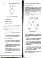
Figure 12.6:
A
map table translates logical to physical addresses
to reserve some bytes to represent the host, others to represent the storage
unit, and so on, a rational address notation would use considerably more than
10
bytes for a system of this scale.
12.3.2 Logical
and
Structured Addresses
One might wonder what the purpose of logical addresses could be. All the infor-
mation needed for
a
physical address is found in the map table, and following
logical pointers to records requires consulting the map table and then going
to the physical address. However, the level of indirection involved in the map
table allows us considerable flexibility. For example, many data organizations
require us to move records around, either within
a
block or from block to block.
If we use a map table, then all pointers to the record refer to this map table,
and all
we have to do when ure move or delete the record is to change the entry
for that record in the table.
Many combinations of logical and physical addresses are possible as well,

yielding
structured
address schemes. For instance, one could use a physical
address for the block (but not the offset within the block), and add the key value
for the record being referred to. Then, to find a record given this structured
address, we use the physical part to reach the block containing that record, and
xe examine the records of the block to find the one with the proper key.
Of course, to survey the records of the block, we need enough information
to locate them. The simplest case is when the records are of a
known, fixed-
length type, with the key field at a known offset. Then, we only have to find in
the block header a count of how many records are in the block, and
xve know
exactly where to find the key fields that might
match the
key
that is part of the
address. However, there axe many other ways that blocks might be organized
so that we could survey the records of the block; we shall cover others shortly.
A
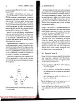
similar, and very useful, combination of physical and logical addresses is
to keep in each block an
oflset table
that holds the offsets of the records within
the
block, as suggested in Fig.
12.7.
Notice that the table grows from the front
end of the block, while the records are placed starting at the end of the block.
This

strategy is useful when the records need not be of equal length. Then, we
12.3.
REPRESENTING
BLOCK
AAiD
RECORD
ADDRESSES
581
do not know in advance how many records the block will hold, and we do not
have to allocate a fixed amount of the block header to the table initially.
offset
-
table-)
header
-'-
unused
-+
record
record
4
record
3
record
1
t
t
I
Figure
12.7:
A

block with a table of offsets telling us the position of each record
within the block
The address of a record is now the physical address of its block plus the offset
of the entry in the block's offset table for that record. This level of indirection
within the block offers many of the advantages of logical addresses, without the
need for a global map table.
1%
can move the record around within the block, and all we have to do
is change the record's entry in the offset table; pointers to the record will
still be able to find it.
We can even allow the record to move to another block, if the offset table
entries are large enough to hold a '.forwarding address" for the record.
Finally, we have an option, should the record be deleted, of leaving in its
offset-table entry
a
tombstone,
a special value that indicates the record has
been deleted. Prior to its deletion, pointers to this record may have been
stored at various places in the database.
After record deletion, following
a pointer to this record leads to the tombstone, whereupon the pointer
can either be replaced by a null pointer, or the data structure otherwise
modified to reflect the deletion of the record. Had we not left the tomb-
stone. the pointer might lead to some new record. with surprising, and
erroneous. results.
12.3.3
Pointer
Swizzling
Often, pointers or addresses are part of records. This situation is not typical
for records that represent tuples of a relation, but it is common for tuples

that represent objects. Also, modern object-relational database systems allow
attributes of pointer type (called references), so
even relational systems need the
ability to represent pointers in tuples. Finally, index structures are composed
of blocks that usually have pointers
within them. Thus, we need to study
Please purchase PDF Split-Merge on www.verypdf.com to remove this watermark.
582
CHAPTER
12.
REPRESENTING DATA ELEMENTS
Ownership
of
Memory Address Spaces
In this section we have presented a view of the transfer between secondary
and main memory in which each client owns its own memory address
space, and the database address space is shared. This model is common
in object-oriented
DBMS's. However, relational systems often treat the
memory address space
as
shared; the motivation is to support recovery
and concurrency
as
we shall discuss in Cliapters 17 and 18.
A
useful compromise is to have a shared memory address space on
the server side, with copies of parts of that space on the clients' side.
That organization supports recovery and concurrency, while also allowing
processing to be distributed in "scalable" way: the more clients the more

processors can be brought to bear.
the management of pointers
as
blocks are moved between main and secondary
memory; we do so in this section.
As
we mentioned earlier, every block, record, object, or other referenceable
data item has two forms of address:
1.
Its address in the server's database address space, which is typically a
sequence of eight or so bytes locating the item in the secondary storage
of the system.
We shall call this address the
database address.
2. An address in virtual memory (provided that item is currently buffered
in virtual memory). These addresses are typically four bytes.
lVe shall
refer to such
an
address
as
the
memory address
of the item.
I?-hen in secondary storage, we surely must use the database address of the
item. However, when the item is in the main
memoiy, we can refer to the item
by either its database address or its memory address. It is more efficient to put
memory addresses wherever an item has a pointer, because these pointers can
be followed using single machine instructions.

In contrast, following a database address is much more time-consuming.
\I-e
need a table that translates from all those database addresses that are currently
'
in virtual memory to their current memory address. Such a
translation table
is
suggested in Fig. 12.8.
It
may be reminiscent of the map table of Fig. 12.6 that
translates
between logical and physical addresses. Ho~vever:
a) Logical and physical addresses are both representations for the database
address. In contrast, memory addresses in the translation table are for
copies of
the corresponding object in memory.
b)
.Ill addressable items in the database have entries in the map table, while
only those items currently in memory are mentioned in the translation
table.
12.3.
R EPRESEiVTIArG BLOCIC AND RECORD ADDRESSES
583
DBaddr mem-addr
database
address
memory
address
Figure 12.8: The translation table turns database addresses into their equiva-
lents in memory

To
a~oid the cost of translating repeatedly from database addresses to mem-
ory addresses, several techniques have been developed that are collectively
known as
pointer swizzling.
The general idea is that when we move a block
from secondary to main memory, pointers within the block may be
"s~vizzled,"
that is, translated from the database address space to the virtual address space.
Thus, a pointer actually consists of:
1.
Al
bit indicating whether the pointer is currently a database address or a
(swizzled) memory address.
2. The database or memory pointer, as appropriate. The same space is used
for
~vllirhever address form is present at the moment. Of course. not all
the space may be used
when the memory address is present, because it is
typically shorter than the database address.
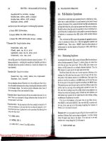
Exatnple
12.7:
Figure 12.9 shoxvs a simple situation in which the Block
1
has
a record
ri-ith pointers to a second record or; the same block and to a record on
another block. The figure also
sho~vs what might happen n-hen Block
1

is copied
to memory. The first pointer. which points within Block
1,
can be stvizzled so
it points directly to the memory address of the target record.
However. if Block
2
is not in memory at this time. then we cannot sn-izzle the
iecond pointer: it must remain unslvizzled. pointing to the database address of
its target. Should Block
2
be brought to memory later. it becomes theoretically
possible
to
swizzle the second pointer of Block 1. Depending on the swizzling
strategy used. there
n~ay or may not be a list of such pointers that are in
memory. referring to Block 2; if
so; then we have the option of sx-izzling the
pointer at that time.
There are several strategies we can use to determine ~vhen to sn-izzle point-
ers.
Please purchase PDF Split-Merge on www.verypdf.com to remove this watermark.
CH-APTER
12.
REPRESENTING DATA
ELEMENTS
Disk
Memory
r8

. . .
.
Read
memory
into
pq
s
Swizzle
Block
1
I
I
Unswizzled
u
Block
2
Figure
12.9:
Structure of a pointer when swizzling is used
Automatic Swizzling
As soon as a block is brought into memory, we locate dl its pointers and
addresses and enter them into the translation table if they are not already
there. These pointers include both the pointers
from
records in the block to
elseivhere and the addresses of the block itself and/or its records. if tliese are
addressable items. We need some mechanism to locate the pointers within the
block. For example:
1.
If the block holds records with a known schema, the schema will tell us

where
in
the records the pointers are found.
2.
If the block is used for one of the index structures we shall discuss in
Chapter
13.
then the block will hold pointers at known locations.
3.
We may keep within the block header a list of where the pointers are.
When we enter into the translation table the addresses for the block just
moved into memory. and/or its records, we know where in memory the block
has been buffered. We ma?; thus create the translation-table entry for tliese
database addresses straightfor~vardly. When
I\-e inscrt one of these database
addresses
-4
into the translatio~l table, we may find it in the table already.
because its block is currently in memory. In this
case,
we replace
-4
in the block
just moved to memory by the corresponding memory address, and
we set the
'.swizzledT bit to true. On the other hand, if
.4
is not yet in the translation
table. then its block has not been copied into main memory.
We therefore

cannot swizzle this pointer and leave it in the block as a database pointer.
12.3.
REPRESENTING
BLOCK
AND
RECORD ADDRESSES
585
If we try to follow a pointer
P
from
a
block, and we find that pointer
P
is
still unswizzled,
i.e., in the form of a database pointer, then we need to niake
sure the block
B
containing the item that
P
points to is in memory (or else
why are we following that pointer?).
We consult the translation table to see if
database address
P
currently has a memory equivalent.
If
not, we copy block
B
into a memory buffer. Once

B
is in memory, we can "swizzle"
P
by replacing
its database form by the equivalent memory form.
Swizzling on
Demand
Another approach is to leave all pointers unswizzled when the block is first
brought into memory.
We enter its address, and the addresses of its pointers,
into the translation table, along with their memory equivalents. If and when
we follow
a
pointer
P
that is inside some block of memory, we swizzle it, using
the same strategy that we followed when we found an unswizzled pointer using
automatic swizzling.
The difference between on-demand and automatic swizzling is that the latter
tries to get all the pointers swizzled quickly and efficiently when the block is
loaded into memory. The possible time saved by swizzling all of a block's
pointers at one time must be weighed against the possibility that some swizzled
pointers will never be followed.
In
that case, any time spent swizzling and
unswizzling the pointer will be wasted.
An interesting option is to arrange that database pointers look like invalid
memory addresses. If so, then we can allow the computer to follow any pointer
as if it
were in its memory form.

If
the pointer happens to be unswizzled, then
the memory reference will cause
a
hardware trap. If the
DBMS
provides a
function that is invoked by the trap, and this function "swizzles" the pointer
in the manner described above, then we can follow swizzled pointers in single
instructions, and only need to do something more time consuming when the
pointer is unswizzled.
No Swizzling
Of course it is possible
newr to swizzle pointers. We still need the translation
table, so the pointers may be followed in their unswizzled form. This approach
does offer the advantage that records cannot be pinned in memory, as discussed
in Section
12.3.5,
and decisions about which form of pointer is present need not
be made.
Programmer Control of Swizzling
In some applications, it may be
known by the application programmer whether
the pointers in
a
block are likely to be follo~ved. This programmer may be able
to specify explicitly that a block loaded into memory is to have its pointers
slvizzled, or the programmer may call for the pointers to be swizzled only
as
needed. For example, if a programmer knows that a block is likely to be accessed

Please purchase PDF Split-Merge on www.verypdf.com to remove this watermark.
586
CHAPTER
12.
REPRESENTING DATA ELEMENTS
heavily, such
as
the root block of a B-tree (discussed in Section 13.3), then the
pointers would be swizzled. However, blocks that are loaded into memory, used
once, and then likely dropped from memory: would not be swizzled.
12.3.4 Returning Blocks
to
Disk
When a block is moved from memory back to disk, any pointers within that
block must be "unswizzled"; that is, their memory addresses must be replaced
by the corresponding database addresses. The translation table can be used
to associate addresses of the two types in either direction, so in principle it is
possible to find, given a memory address, the database address to which the
memory address is assigned.
However, we do not want each unswizzling operation to require a search of
the entire translation table. While we have not discussed the implementation of
this table, we might imagine that the table of Fig.
12.8
has appropriate indexes.
If we think of the translation table
as
a relation, then the problem of finding
the memory address associated with a database address
x
can be expressed as

the query:
SELECT memAddr
FROM
TranslationTable
WHERE
dbAddr
=
x;
For instance, a hash table using the database address
as
the key might be
appropriate for an index on the
dbAddr
attribute; Chapter
13
suggests many
possible data structures.
If we want to support the reverse query,
SELECT dbAddr
FROM
TranslationTable
WHERE
memAddr
=
y;
then ~c-e need to have an index on attribute
memAddr
as
well. Again, Chapter 13
suggests data structures suitable for such an index.

Also, Section 12.3.5 talks
about linked-list structures that in some circumstances can be used to go from
a memory address to all main-memory pointers to that address.
12.3.5 Pinned Records
and
Blocks
A
block in memory is said to be
pinned
if it cannot at the moment be written
back to
disk safely.
A
bit telling whether or not a block is pinned can be located
in the header of the block. There are many reasons
why a block could be pinned,
including requirements of a recovery system
as
discussed in Chapter
17.
Pointer
swizzling introduces an important reason why certain blocks must be pinned.
If a block
B1
has within it a swizzled pointer to some data item in block
Bg,
then n-e must be very careful about moving block
B2
back to disk and reusing
12.3.

REPRESENTING BLOCK AND RECORD ADDRESSES
587
its main-memory buffer. The reason is that, should we follow the pointer in
B1,
it
will lead us to the buffer, which no longer holds
Bz;
in effect, the pointer
has become dangling. A block, like
B2,
that is referred to by a swizzled pointer
from somewhere else is therefore pinned.
When
we write a block back to disk, we not only need to "unswizzle" any
pointers in that block.
We also need to make sure it is not pinned.
If it is
pinned, we must either unpin it, or let the block remain in memory, occupying
space that could otherwise be used for some other block. To unpin a block
that is pinned because of swizzled pointers from outside, we
xllust "unswizzle"
any pointers to it. Consequently, the translation table must record, for each
database address whose data item is in memory, the places in memory where
swizzled pointers to that item exist.
TWO possible approaches are:
1.
Keep the list of references to a memory address as a linked list attached
to
the
entry for that address in the translation table.

2.
If memory addresses are significantly shorter than database addresses, we
can create the linked list in the space used for the pointers themselves.
That is, each space used for a database pointer is replaced by
(a) The swizzled pointer, and
(b) Another pointer that forms part of a linked list of all occurrences of
this pointer.
Figure 12.10 suggests
how all the occurrences of a memory pointer
y
could be linked, starting at the entry in the translation table for database
address
x
and its corresponding memory address
y.
I
Swizzled pointer
Translation table
Figure 12.10:
.A
linked list of occurrences of a swizzled pointer
12.3.6 Exercises for Section 12.3
*
Exercise
12.3.1
:
If we represent physical addresses for the Megatron
747
disk
by allocating a separate byte or bytes to each of the cylinder, track

within
Please purchase PDF Split-Merge on www.verypdf.com to remove this watermark.
588
CHAPTER
12.
REPRESENTING
DATA
ELE114E1VTS
a cylinder, and block within a track, how many bytes do we need? Make a
reasonable assumption about the maximum number of blocks on each track;
recall that the Megatron
747 has
a
variable number of sectorsltrack.
Exercise 12.3.2: Repeat Exercise 12.3.1 for the Megatron 777 disk described
in Exercise 11.3.1
Exercise 12.3.3:
I£
we wish to represent record addresses as well as block
addresses, we need additional bytes. Assuming we want addresses for a single
Megatron 747 disk
as
in Exercise 12.3.1, how many bytes would we need for
record addresses if we:
*
a) Included the number of the byte within a block as part of the physical
address.
b) Used structured addresses for records. Assume that the stored records
have a 4-byte integer
as

a key.
Exercise 12.3.4: Today, IP addresses have four bytes. Suppose that block
addresses for a world-wide address system consist of an
IP
address for the host,
a device number between
1
and 1000, and a block address on an individual
device (assumed to be a Megatron 747 disk). How many bytes would block
.
addresses require?
Exercise 12.3.5
:
In IP version 6, IP addresses are 16 bytes long. In addition,
we may want to address not only blocks, but records, which may start at any
byte of
a
block. However, devices will have their own IP address, so there will
be no
need
to represent a device within a host,
as
we suggested
was
necessary
in Exercise 12.3.4. How many bytes
would be needed to represent addresses in
these circumstances, again assuming devices were
Xegatron 747 disks?
!

Exercise 12.3.6: Suppose we wish to represent the addresses of blocks on a
Megatron 747 disk logically,
i.e., using identifiers of
k
bytes for some
k.
We also
need to store on the disk itself a map table,
as
in
Fig.
12.6, consisting of pairs
of
logical and physical addresses. The blocks used for the map table itself are
not part of the database, and therefore do not have their own logical addresses
in the map table. Assuming that physical addresses use the minimum possible
number of bytes for physical addresses
(as
calculated in Exercise 12.3.1), and
logical addresses likewise use the minimum possible number of bytes for logical
addresses, how many blocks of 4096 bytes does the map table for the disk
occupy?
*!
Exercise
12.3.7:
Suppose that we have 4096-byte blocks in which wve store
records of 100 bytes. The block header consists of an offset table, as in Fig. 12.7.
using 2-byte pointers to records within the block. On
an
average day. two

records per block are inserted, and one record is deleted.
h
deleted record must
have its pointer replaced by a "tombstone," because there may be
da~lgling
I
12.4.
VARI-4BLGLEArGTH
DATA
AAD RECORDS
589
pointers to it. For specificity, assume the deletion on any day always occurs
before the insertions. If the block is initially empty, after how many days will
there be no room to insert any more records?
!
Exercise 12.3.8: Repeat Exercise 12.3.7 on the assumption that each day
there
is
one deletion and 1.1 insertions on the average.
Exercise
12.3.9:
Repeat Exercise 12.3.7 on the assumption that instead of
deleting records, they are mored to another block and must be given an 8-byte
forwarding address in their offset-table entry. Assume either:
!
a) All offset-table entries are given the maximum number of bytes needed in
an entry.
!!
b) Offset-table entries are allowed
to

vary in length in such a way that all
entries can be found and interpreted properly.
*
Exercise 12.3.10: Suppose that if we swizzle all pointers automatically, we
can perform the swizzling in half the time it would take to swizzle each one
separately. If the probability that a pointer in main
memory xvill be followed at
least once is
p,
for what values of
p
is it more efficient to swizzle automatically
than on demand?
!
Exercise 12.3.11
:
Generalize Exercise 12.3.10 to include the possibility that
we never swizzle pointers. Suppose that the important actions take the following
times, in some arbitrary time units:
i.
On-demand swizzling of a pointer: 30.
ii.
dutomatic swizzling of pointers: 20 per pointer.
iii.
Following a sn-izzled pointer:
1.
iv.
Following an unswizzled pointer: 10.
Suppose that in-memory pointers are either not
follorved (probability 1

-
p)
or are follon-ed
k
times (probability
p).
For what values of
k
and
p
do no-
srvizzling, automatic-swizzling, and on-demand-sn-izzling each offer the best
average performance?
12.4
Variable-Length Data
and
Records
Until now, we have made the simplifying assumptions that every data item has
a
fised length, that records have a fixed schema, and that the schema is a list of
fixed-length fields.
Howerer, in practice, life is rarely so simple. We may wish
to represent:
Please purchase PDF Split-Merge on www.verypdf.com to remove this watermark.
590
CHAPTER
12.
REPRESENTING DATA ELEMENTS
1.
Data items whose size varies.

For instance, in Fig. 12.1 we considered a
Moviestar relation that had an address field of up to
255
bytes. While
there might be some addresses that long, the vast majority of them will
probably be
50
bytes or less. We could probably save more than half the
space used for storing
MovieStar tuples if we used only as much space
as
the actual address needed.
2.
Repeating fields.
If we try to represent a many-many relationship in a
record representing an object, we shall have to store references to as many
objects as are related to the given object.
3.
Variable-format records.
Sometimes we do not know in advance what the
fields of a record will be, or how many occurrences of each field there
will be. For example, some movie stars also direct movies, and
we might
want to add fields to their record referring to the movies they directed.
Likewise, some stars produce movies or participate in other ways, and we
might wish to put this information into their record
as
well.
However,
since most stars are neither producers nor directors, we would not want

to reserve space for this information in every star's record.
4.
Enormous fields.
Modern DBMS's support attributes whose value is a
very large data item. For instance, we might want to include a picture
attribute with a movie-star record that is a GIF image of the star.
-1
movie record might have a field that is a 2-gigabyte
MPEG
encoding of
the movie itself,
as
well
as
more mundane fields such as the title of the
movie. These fields are so large, that our intuition that records fit within
blocks is contradicted.
12.4.1
Records With Variable-Length Fields
If one or more fields of a record have variable length, then the record must
contain enough information to let us find any field of the record.
A
simple
but effective scheme is to put all fixed-length fields ahead of the variable-length
fields.
We then place in the record header:
1.
The length of the record.
2.
Pointers to (i.e., offsets of) the beginnings of all the variable-length fields.

However, if the
variable-length fields always appear in the same order.
then the first of them needs no pointer; we
know it immediately follo~vs
the fiscd-length fields.
Example
12.8:
Suppose that w-e have movie-star records with name, address:
gender, and birthdate.
\Ve shall assume that the gender and birthdate are
fixed-length fields, taking
4
and 12 bytes, respectively. However, both name
and address will be represented by character strings of
xhatever length is
ap-
propriate. Figure 12.11 suggests what a typical movie-star record would look
12.4.
T'I1RIABLELENGTH
DATA
AND
RECORDS
591
like. We shall always put the name before the address. Thus, no pointer to
the beginning of the name is needed; that field will always begin right after the
fixed-length portion of the record.
0
other header information
record length
to address

I
Ill


.
, ,
ibirthdate
j
name
i
address
. . . .


Figure 12.11:
A
MovieStar record with
name
and
address
implemented
as
variable-length character strings
12.4.2
Records With Repeating Fields
A
similar situation occurs if a record contains
a
variable number of occurrences
of a field

F,
but the field itself is of fixed length. It
is
sufficient to group all
occurrences of field
F
together and put in the record header a pointer to the
first.
We can locate all the occurrences of the field
F
as follows. Let the number
of bytes
del-oted to one instance of field
F
be
L.
We then add to the offset for
the field
F
all integer multiples of
L,
starting at
0,
then
L,
2L,
3L,
and so on.
Eventually, we reach the offset of the field following
F.

whereupon we stop.
other header information
record length
to address
I
,
to movie pointers
1
I.'.'.

. .
.
.
,
. .
t'tit.
. .
.
.
.
. .
.
. . .
.
. .
. .
.

,
,

.
.
:
name
i
address
i
.
i
i
i
i i
i
;

.
. . . . .
,
,
.
,
. .
.
.
.
,

.,
L
A

-
pointers to movies
Figure 12.12:
-1
record with a repeating group of references to movies
Example
12.9
:
Suppose that we redesign our movie-star records to hold only
the name and address (which are variable-length strings) and pointers to all
the movies of the star. Figure 12.12 shows how this type of record could be
represented. The header contains pointers to the beginning of the address
fieid
(we assume the name field always begins right after the header) and to the
Please purchase PDF Split-Merge on www.verypdf.com to remove this watermark.
.
592
CHAPTER
12.
REPRESENTING
DATA
ELEMENTS
Representing
Null
Values
Tuples often have fields that may be
NULL.
The record format of Fig.
12.11
offers a convenient way to represent

NULL
values.
If
a field such
as
address
is null, then we put
a
null pointer in the place where the pointer to an
address goes. Then, we need no space for an address, except the place for
the pointer. This arrangement can save space on average, even if address
is a fixed-length field but frequently has the value
NULL.
first of the movie pointers. The length of the record tells us how many movie
pointers there are.
An
alternative representation is to keep the record of fixed length, and put
the
variabklength portion
-
be it fields of variable length or fields that sepeat
an indefinite number of times
-
on
a
separate block. In the record itself we
keep:
1.
Pointers to the place where each repeating field begins, and
2.

Either how many repetitions there are, or where the repetitions end.
Figure
12.13
shows the layout of a record for the problem of Example
12.9,
but with the variable-length fields name and address, and the repeating field
starredrn (a set of movie references) kept on a separate block or blocks.
There are advantages and disadvantages to using indirection for the
variable-
length components of a record:
Keeping the record itself fixed-length allows records to be searched more
efficiently, minimizes the overhead in block headers, and allows records to
be moved
within or among blocks with minimum effort.
On the other hand, storing variable-length components on another block
increases the number of disk
I/07s needed to examine all components of
a record.
A
compromise strategy is to keep in the fixed-length portion of the record
enough space for:
1.
Some reasonable number of occurrences of the repeating fields,
2. A
pointer to a place where additional occurrences could be found, and
3.
X
count of how many additional occurrences there are.
If there are fewer than this number, some of the space would be unused. If there
are more than can fit in the fixed-length portion, then the pointer to additional

space will be nonnull, and we can find the additional occurrences by following
this pointer.
12.4.
K4RIABLELENGTH
DATA
AND
RECORDS
I
record header information
I
to name
length of name
to address
length of address
to movie references
Record





address

name
Additional space
Figure
12.13:
Storing variable-length fields separately from the record
12.4.3
Variable-Format Records

An even more complex situation occurs when records do not have a fixed
schema. That is, the fields or their order are not completely determined by
the relation or class whose tuple or object the record represents. The simplest
representation of sariable-format records is a sequence of
tagged fields,
each of
which consists of:
1.
Information
about the role of this field, such
as:
(a) The attribute or field name,
(b) The type of
the
field, if it is not apparent from the field name and
some readily available schema information, and
(c) The length of the field, if it is not apparent from the type.
2.
The value of the field.
There are at least
tn-o reasons why tagged fields would make sense.
1.
Information-integration applicattons.
Sometimes, a relation has been con-
structed from several earlier sources, and these sources
hare different kinds
of information; see Section
20.1
for
a

discussion. For instance, our niovie-
star information may ha~e come from several sources, one of which records
birthdates and the others do not, some
gire addresses, others not, and so
on.
If
there are not too many fields, 1%-e are probably best off leaving
NULL
Please purchase PDF Split-Merge on www.verypdf.com to remove this watermark.
594
CHAPTER
12.
REPRESENTING DATA ELEMENTS
those values we do not know. However, if there are many sources, with
many different kinds of information, then there may be too many
NULL'S,
and we can save significant space by tagging and listing only the nonnull
fields.
2.
Records
with
a very flexible schema.
If many fields of a record can repeat
and/or not appear at all, then even if we know the schema, tagged fields
may be useful. For instance, medical records may contain information
about many tests, but there are thousands of possible tests, and each
patient has results for relatively few of them.
Example
12.10
:

Suppose some movie stars have information such as movies
directed, former spouses, restaurants owned, and a number of other fixed but
unusual pieces of information. In Fig.
12.14
we see the beginning of a hypothet-
ical
movie-star record using tagged fields. We suppose that single-byte codes
are used for the various possible field names and types. Appropriate codes are
indicated on the figure, along with lengths for the two fields shown, both of
which happen to be of type string.
I
code for name
1
code for restaurant owned
code for string
type
code for string
type
1
length
7
length

,
.
,,.
.

.

.

.
N;

s
j
14;
.
Clint
~astwood
R!
S;
16;
Hog's Breath
1%
,.
.

.
.

.
.,.
.
Figure
12.14:
A
record with tagged fields
12.4.4

Records That
Do
Not
Fit
in
a
Block
We shall now address another problem whose importance has been increasing
as
DBMS's are more frequently used to manage datatypes with large values:
often values do not fit in one block. Typical examples are video or audio "clips."
Often, these large values have
a
vaiiable length, but even if the length is fixed
for all values of the type, we need to use some special techniques to represent
these values. In this section we shall consider a technique called
'.spanned
records" that can be used to manage records that are larger than blocks. The
management of extremely large values (megabytes or gigabytes) is addressed in
Section
12.4.5.
Spanned records also are useful in situations where records are smaller than
blocks, but packing whole records into blocks wastes significant amounts of
space. For instance, the waste space in Example
12.6
was only
7%,
but if
records are just slightly larger than half a block, the wasted space can approach
50%.

The reason is that then we can pack only one record per block.
12.4.
VARIABLELENGTH D.4TA AND RECORDS
595
For both these reasons, it is sometimes desirable to allow records to be split
across two or more blocks. The portion of a record that appears in one block is
called a
record fragment.
A record with two or more fragments is called
spanned,
and records that do not cross a block boundary are
unspanned.
If records can be spanned, then every record and record fragment requires
some extra header information:
1.
Each record or fragment header must contain a bit telling whether or not
it is a fragment.
2.
If it is a fragment, then it needs bits telling whether it is the first or last
fragment for its record.
3.
If there is a next and/or previous fragment for the same record, then the
fragment needs pointers to these
ot,her fragments.
Example
12.11:
Figure
12.15
suggests how records that were about
GO%

of a
block in size could be stored with three records for every two blocks. The header
for record fragment
2a
contains an indicator that it is a fragment, an indicator
that it is the first fragment for its record, and a pointer to nest fragment,
2b.
Similarly, the header for
2b
indicates it is the last fragment for its record and
holds a back-pointer to the previous fragment
2a.
block header
block
1 block 2
Figure
12.15:
Storing spanned records across blocks
:
recor
I
i
2-bd
12.4.5
BLOBS
i
;
record
3
Xow, let us consider the representation of truly large values for records or fields

of records. The common esamples include images in
~arious formats (e.g., GIF,
or JPEG), movies in formats such as
IIPEG, or signals of all sorts: audio, radar,
and so on. Such values are often called
binary, large objects,
or BLOBS. When
a field has a
BLOB
as value, we must rethink at least two issues.
t
Please purchase PDF Split-Merge on www.verypdf.com to remove this watermark.
CHAPTER
12.
REPRESENTIArG DATA ELEMENTS
Storage
of
BLOBS
A
BLOB must be stored on a sequence of blocks. Often we prefer that these
blocks are allocated consecutively on
a
cylinder or cylinders of the disk, so the
BLOB may be retrieved efficiently. However, it is also possible to store the
BLOB on a linked list of blocks.
lloreo\rer, it is possible that the BLOB needs to be retrieved so quickly
(e.g., a movie that must be played in real time), that storing it on one disk
does not allow us to retrieve it fast enough. Then, it is necessary to
stripe
the

BLOB across several disks, that is, to alternate blocks of the BLOB among
these disks. Thus, several blocks of the BLOB can be retrieved simultaneously.
increasing the retrieval rate by a factor approximately equal to the number of
disks involved in the striping.
Retrieval
of
BLOBS
Our assumption that when a client wants a record, the block containing the
record is passed from the database server to the client in its entirety may not
hold. We may want to pass only the "small" fields of the record, and allow the
client to request blocks of the BLOB one at a time, independently of the rest of
the record. For instance, if the BLOB is
a
2-hour movie, and the client requests
that the movie be played, the BLOB could be shipped several blocks at a time
to the client, at just the rate necessary to play the movie.
In many applications, it is also important that the client be able to request
interior portions of the BLOB without having to receive the entire BLOB.
Examples would be a request to see the 45th minute of a movie, or the ending
of an audio clip. If the
DBMS is to support such operations, then it requires a
suitable index structure,
e.g., an index by seconds on a movie BLOB.
12.4.6
Exercises for Section
12.4
*
Exercise
12.4.1
:

.A
patient record consists of the follolving fixed-length fields:
the patient's date of birth, social-security number, and patient ID,
each 10 bytes
long. It also has the following variable-length fields: name, address, and patient
history. If pointers within a record require
4
bytes, and the record length is a
$-byte integer, how many bytes. esclusire of the space needed for the variable-
length fields, are needed for the record? You may assume that no alignment of
fields is required.
*
Exercise
12.4.2:
Suppose records arc
as
in Exercise 12.4.1, and the variable-
length fields
name. address. and history each have a length that is unifornlly
distributed. For the name. the range is 10-30 bytes; for address it is 20-80
bytes, and for history it is 0-1000 bytes.
What is the average length of a
patient record?
Exercise
12.4.3:
Suppose that the patient records of Exercise 12.4.1 are aug-
mented by an additional repeating field that represents cholesterol tests.
Each
12.4.
VARIABLE-LENGTH DAT4 -4iVD RECORDS

597
cholesterol test requires 16 bytes for a date and an integer result of the test.
Show the layout of patient records if:
a) The repeating tests are kept with the record itself.
b) The tests are stored on a separate block, with pointers to them in the
record.
Exercise
12.4.4
:
Starting with the patient records of Exercise 12.4.1, suppose
we add fields for tests and their results. Each test consists of a test name, a
date, and a test result. Assume that each such test requires 40 bytes. Also,
suppose that for each patient and each test a result is stored with probability
P.
a) Assuming pointers and integers each require 4 bytes, what is the average
number of bytes devoted to test results in a patient record, assuming that
all test results are kept within the record itself, as a variable-length field?
b) Repeat (a), if test results are represented by pointers within the record
to test-result fields kept
elselvhere.
!
c) Suppose we use a hybrid scheme, where room for
k
test results are kept
within the record, and additional test results are found by following a
pointer to another block (or chain of blocks) where those results are kept.
As a function of
p.
what value of
k

minimizes the amount of storage used
for
test results?
!!
d) The antount of space used by the repeating test-result fields is not the
only issue. Let us suppose that the figure of merit 1%-e wish to minimize
is the number of bytes used. plus a penalty of 10,000 if we have to store
some results on another block (and therefore will require a disk
I/O for
many of the test-result accesses
we need to do. Under this assumption,
what is the best
value of
k
as a function of
p?
*!!
Exercise
12.4.5:
Suppose blocks have 1000 bytes available for the storage of
records, and
1%-e wish to store on them fixed-length records of length r, where
500
<
r
5
1000. The value of r includes the record header, but a record
fragment requires an additional 16 bytes for the fragment header. For what
values of r can
we improve space utilization by spanning records?

!!
Exercise
12.4.6:
An
NPEG
movie uses about one gigahyte per hour of play.
If
we carefully organized several mox-ies on a Megatron
747
disk, ho~v many
could we deliver with only small delay (say 100 milliseconds) from one disk.
Use the
tinling estimates of Example 11.5: but remember that
)pu
can choose
how the movies are laid out on the disk.
Please purchase PDF Split-Merge on www.verypdf.com to remove this watermark.
598
CHAPTER
12.
REPRESENTING DATA ELEMENTS
12.5
Record Modifications
Insertions, deletions, and update of records often create special problems. These
problems are most severe when the records change their length, but they
come
up even when records and fields are all of fixed length.
12.5.1
Insertion
First, let us consider insertion of new records into a relation (or equivalently,

into the current extent of a class). If the records of a relation are kept in
no particular order,
we can just find a block with some empty space, or get
a new block if there is none, and put the record there. Usually, there is some
mechanism for finding all the blocks holding tuples of
a
given relation or objects
of a class, but we shall defer the question of how to keep track of these blocks
until. Section
13.1.
There is more of a problem when the tuples must be kept in some fixed
order, such
as
sorted by their primary key. There is good reason to keep records
sorted, since it facilitates answering certain kinds of queries,
as
we shall see in
Section
13.1.
If
we need to insert a new record, we first locate the appropriate
block for that record. Fortuitously, there may be space in the block to put the
new record. Since records must be kept in order, we may have to slide records
around in the block to make space available at the proper point.
If we need to slide records, then the block organization that me showed in
Fig.
12.7,
which we reproduce here as Fig.
12.16,
is

useful. Recall from our
discussion in Section
12.3.2
that we may create an "offset table" in the header
of each block, with pointers to the location of each record in the block. A
pointer to
a
record from outside the block is
a
"structured address," that is,
the block address and the location of the entry for the record in the offset table.
offset
-
table-)
+
header
tf
unused
-
-
record
record
4
record
3
record
1
4
C
4

Figure
12.16:
An offset table lets us slide records xithin a block to ilinke room
for new records
If
we can find room for the inserted record in
the
block at hand, then we
simply slide the records within the block and adjust the pointers in the offset
table. The new record is inserted into the block, and a new pointer to the
record is added to the offset table for the block.
12.5.
RECORD MODIFlCATlONS
599
However, there may be no room in the block for the new record, in which
case we have to find room outside the block. There are two major approaches
to solving this problem, as well as combinations of these approaches.
1.
Find space on a "nearby" block.
For example, if block B1 has no available
space.for a record that needs to be inserted in sorted order into that block,
then look at the following block
B2 in the sorted order of the blocks. If
there is room in
B2,
move the highest record(s) of B1 to B2, and slide the
records around on both blocks. However, if there are external pointers to
records, then we have to be careful to leave a
forwarding address
in the

offset table of
B1 to say that a certain record has been moved to Bz and
where its entry in the offset table of
B2 is. Allowing forwarding addresses
typically increases the amount of space needed for entries of the offset
table.
2.
Create an overflow block.
In this scheme, each block
B
has in its header
a place for a pointer to an
overflow
block where additional records that
theoretically belong in
B
can be placed. The overflow block for
B
can
point to a second overflow block, and so on. Figure
12.17
suggests the
structure.
We show the pointer for overflow blocks
as
a nub on the block,
although it is in fact part of the block header.
Block
B
overflow block

for
B
Figure
12.17:
A
block and its first overflow block
12.5.2
Deletion
When we delete a record,
we
may be able to reclaim its space. If we use an
offset table as in Fig.
12.16
and records can slide around the block. then we
can compact the space in the block so there is aln-ays one unused region in the
center. as suggested by that figure.
If
we cannot slide records,
we
should maintain an available-space list in the
block header. Then
we shall knon where. arid how large, the available regions
are, n-hen a
new record is inserted into the block. Sote that the block header
normally does
not need to hold the entire available space list. It is sufficient to
put the list head in the block header, and use the available regions
themsell-es
to hold the links in the list. much as we did in Fig.
12.10.

When a record is deleted, we may be able to do away with an overflow block.
If the record is deleted either from a block
B
or from any block on its overflow
Please purchase PDF Split-Merge on www.verypdf.com to remove this watermark.
600
CHAPTER
12.
REPRESENTING D.4TA ELEMENTS
chain, we can consider the total amount of used space on all the blocks of that
chain. If the records can fit on fewer blocks, and we can safely move records
among blocks of the chain, then a reorganization of the entire chain can be
performed.
However, there is one additional complication involved in deletion, which
we
must remember regardless of what scheme we use for reorganizing blocks. There
may be pointers to the deleted record, and if so,
we don't want these pointers
to dangle or wind up pointing to a new record that
is
put in the place of the
deleted record. The usual technique, which
we pointed out in Section 12.3.2, is
to place a
tombstone
in place of the record. This tombstone is permanent; it
must exist until the entire database is reconstructed.
Where the tombstone is placed depends on the nature of record pointers.
If pointers go
to

fixed locations from which the location of the record is found,
then
we put the tombstone in that fixed location. Here are two examples:
1.
We suggested in Section 12.3.2 that if the offset-table scheme of Fig. 12.16
were used, then the tombstone could be a null pointer in the offset table,
since pointers to the record were really pointers to the offset table entries.
2.
If we are using a map table, as in Fig. 12.6, to translate logical record
addresses to physical addresses, then the tombstone can be a null pointer
in place of the physical address.
If
we need to replace records by tombstones, it would be wise to have at the
very beginning of the record header a bit that serves as
a
tombstone; i.e., it is
0
if the record is
not
deleted, while
1
means that the record has been deleted.
Then, only this bit must remain where the record used to begin, and subsequent
bytes can be reused for another record,
as
suggested by Fig. 12.18.~ \$'hen we
follow
a
pointer to the deleted record, the first thing we see is the "tombstone"
bit telling us that the record was deleted. We then

know not to look at the
following bytes.
t
1
i
record
2
Figure 12.18: Record
1
can be replaced, but the tombstone remains: record
2
has no tombstone and can be seen when we follow
a
pointer to it
3~o~ve\.er, the field-alignment problem discussed in Section 12.2.1 may force
us
to leave
four bytes or more
unused.
12.5.
RECORD MODIFIC.~TIOIYS
12.5.3 Update
When a fixed-length record is updated, there is no effect on the storage system,
because we know it can occupy exactly the same space it did before the update.
However, when a variable-length record is updated, we have all the problems
associated with both insertion and deletion, except that it is never necessary to
create a tombstone for the old version of the record.
If the updated record is longer than the old version, then we map
need
to create more space on its block. This process may involve sliding records

or
even the creation of an overflow block. If variable-length portions of the
record are stored on another block,
as
in Fig. 12.13, then we may need to move
elements around that block or create a new block for storing variable-length
fields. Conversely, if the record shrinks because of the update, me have the
same opportunities
as
with a deletion to recover or consolidate space, or to
eliminate overflow blocks.
12.5.4 Exercises for Section 12.5
Exercise
12.5.1
:
Suppose we have blocks of records sorted by their sort key
field and partitioned among blocks in order. Each block has a range of sort
keys that is known from outside (the sparse-index structure in Section
13.1.3 is
an example of this situation). There are no pointers to records from outside, so
it is possible to move records between blocks if
\ye wish. Here are some of the
ways
we could manage insertions and deletions.
i.
Split blocks whenever there is an overflow. Adjust the range of sort keys
for a block when
we do.
ii. Keep the range of sort keys for a block fixed: and use
overflow blocks as

needed. Keep for each block and each overflow block an offset table for
the records in that block alone.
iii. Same as (ii), but keep the offset table for the block and all its
overflow
blocks in the first block (or overflow blocks if the offset table needs the
space). Note that if
more space for the offset table is needed. n-e can move
records from the first block to an overflow block to make
room.
iv.
Same
as
(ii), but keep the sort key along. n-ith a pointer in the offset
tables.
2:.
Same as (iii); but keep the sort key along with a pointer in the offset
table.
-1nslver the following questions:
*
a) Compare methods
(i)
and
(ii)
for the average numbers of disk 110's
needed to retrieve the record, once the block (or first block in a chain
with overflow blocks) that could have a record 1~-ith a given sort key is
Please purchase PDF Split-Merge on www.verypdf.com to remove this watermark.
CHAPTER
12.
REPRESEXTING DATA ELEhIEiVTS

found. Are there any disadvantages to the method with the fewer average
disk
I/O's?
b) Compare methods (ii) and (iib) for their average numbers of disk 110's per
record
retrival,
as
a function of
b,
the total number of blocks in the chain.
Assume that the offset table takes
10%
of the space, and the records take
the remaining
90%.
!
c) Include methods (iv) and (v) in the comparison from part
(b).
Assume
that the sort key is
119
of the record. Note that we do not have to repeat
the sort key in the record if it is in the offset table. Thus, in effect, the
offset table uses
20%
of the space and the remainders of the records use
80%
of the space.
Exercise
12.5.2

:
Relational database systems have always preferred to use
fixed-length tuples if possible. Give three reasons for this preference.
l2.6
Summary
of
Chapter
12
+
Fields:
Fields are the most primitive data elements. Many, such as in-
tegers or fixed-length character strings, are simply given an appropriate
number of bytes in secondary storage. Variable-length character strings
are stored either in a fixed sequence of bytes containing an endmarker,
or in an area for varying strings, with a length indicated by an integer at
the beginning or an endmarker at the end.
+
Records:
Records are composed of several fields plus a record header. The
header contains information about the record, possibly including such
matters
as
a timestamp, schema information, and a record length.
+
Variable-Length Records:
If records contain one or more variable-length
fields or contain
an
unknown number of repetitions of a field, then addi-
tional structure is necessary. A directory of pointers in the record header

can be used to locate variable-length fields within the record. Alterna-
tively, we can replace the variable-length or repeating fields by
(fised-
length) pointers to a place outside the record where the field's value is
kept.
+
Blocks:
Records are generally stored within blocks.
A
block header. with
information about that block. consumes some of the space in the block.
I\-ith the remainder occupied by one or more records.
+
Spanned Records:
Generally, a record exists within one block. However,
if records are longer than blocks, or we wish to make use of left,over space
nithin blocks, then we can break records into two or more fragments, one
on each block.
!
fragment header is then needed to
link
the fragments of
a
record.
12.7.
REFERENCES FOR CHAPTER
12
603
+
BLOBS:

Very large values, such
as
images and videos, are called BLOBS
(binary, large objects). These values must be stored across many blocks.
Depending on the requirements for access, it may be desirable to keep the
BLOB on one cylinder, to reduce the access time for the BLOB, or it may
be necessary to stripe the
BLOB
across several disks, to allow parallel
retrieval of its
content.%
+
Offset Tables:
To support insertions and deletions of records,
as
well as
records that change their length due to modification of varying-length
fields, we can put in the block header an offset table that has pointers to
each of the records in the block.
+
Overflow Blocks:
Also to support insertions and growing records, a block
may have a link to
an
overflow block or chain of blocks, wherein are kept
some records that logically belong in the first block.
+
Database Addresses:
Data managed by a DBMS is found among several
storage devices, typically disks. To locate blocks and records in this stor-

age system, we can use physical addresses, which are a description of
the device number, cylinder, track,
sector(s), and possibly byte within a
sector.
We can also use logical addresses, which are arbitrary character
strings that are translated into physical addresses by a map table.
+
Structured Addresses:
We may also locate records by using part of the
physical address,
e.g., the location of the block whereon a record is found,
plus additional information such as a key for the record or a position in
the offset table of
a
block that locates the record.
+
Pointer
Swizzling:
When disk blocks are brought to main memory, the
database addresses need to be translated to memory addresses, if pointers
are to be followed. The translation is called swizzling, and can either be
done automatically, when blocks are brought to memory, or on-demand,
when a pointer is first followed.
+
Tombstones:
When a record is deleted, pointers to it will dangle.
A
tombstone in place of (part of) the deleted record warns the system that
the record is no longer there.
+

Pinned Blocks:
For various reasons, including the fact that a block may
contain swizzled pointers, it may be unacceptable to copy a block from
memory back to its place on disk. Such a block is said to be pinned. If the
pinning is due to
slvizzled pointers. then they must be unswizzled before
returning the block to disk.
12.7
References
for
Chapter
12
The classic
1968
text on the subject of data structures
[2]
has been updated
recently.
[.I]
has information on structures relevant to this chapter and also
Please purchase PDF Split-Merge on www.verypdf.com to remove this watermark.
CHAPTER
12.
REPRESENTING
DATA
ELEMENTS
Chapter
13.
Tombstoner
as

a technique for dealing with deletion is from
[3]. [I]
covers
data reoresentation issues, such
as
addresses and swizzling in the context of

object-oriented DBMS's.
1.
.
.
G.
Cattell,
Object Data Management,
Addison-Wesley, Reading
?VIA,
1994.
2.
D.
E.
Knuth,
The Art of Computer Programming,
Vol.
I,
Fundamental
Algorithms,
Third
Edition,
Addison-Wesley, Reading
M.4,

1997.
3.
D.
Lomet, "Scheme for invalidating free references,"
IBM
J.
Research and
Development
19:l
(1975),
pp.
26-35.
4.
G. Wiederhold,
File Organization for Database Design,
McGraw-Hill,
New York,
1987.
Index
Structures
Having seen the options available for representing records, we must now consider
how whole relations, or the extents of classes, are represented. It is not sufficient
simply to scatter the records that represent tuples of the relation or objects
of the extent
aniong various blocks. To see mhy, ask how Ive would answer
even the simplest query, such as
SELECT
*
FROM
R.

ifre would have to examine
every block in the storage system and hope there is enough information in block
headers to identify
where in the block records begin and enough information in
record headers to tell in
what relation the record belongs.
A
slightly better organization is to reserve some blocks, perhaps several
xvhole cylinders, for a given relation.
All blocks in those cylinders may be
assumed to hold records that represent tuples of our relation. Now; at least we
can find the tuples of the relation without scanning the entire data store.
However. this organization offers no
help should we want to answer the
next-simplest query, such
as
SELECT
*
FROM
R
WHERE
a=10.
Section
6.6.6
in-
troduced us to the importance of creating
indexes
on a relation, in order to
speed up the discovery of those tuples of a relation that have a particular value
for a particular attribute. As suggested in Fig.

13.1.
an index is any data struc-
ture that takes
as
input a property of records
-
typically the value of one or
more fields
-
and finds the records with that property "quickly." In particu-
lar, an index lets us find a record without having to look at more than a small
fraction of all possible records. The
field(s) on whose values the index is based
is called the
search key.
or just "key" if the index is understood.
Many different data structures can serve as indexes.
In the remainder of
this chapter
n.e consider the follo~\-ing methods:
1.
Simple indexes on sorted files.
2.
Secondary indexes on unsorted files.
3.
B-trees, a commonly used way to build indexes on any file.
4.
Hash tables, another useful and important index structure.
Please purchase PDF Split-Merge on www.verypdf.com to remove this watermark.
CHAPTER

13.
INDEX
STRUCTURES
13.1.
11vDEXES
ON
SEQ
UENTML
FILES
value
-+
Index
)
records
-
records
Figure
13.1:
An index takes a value for some field(s) and finds records with the
matching value
Keys and More Keys
There are many meanings of the term "key." We used it in Section
7.1.1
to mean the primary key of a relation. In Section
11.4.4
we learned about
Figure
13.2:
-4
sequential file

.'sort keys," the attribute(s) on which
a
file of records is sorted. Now,
we shall speak of "search keys," the attribute(s) for which we are given
values and
asked to search, through an index, for tuples with matching
In this file, the tuples are sorted by their primary key.
IVe imagine that keys
\ralues. We try to use the appropriate adjective
-
"primary," "sort," or
are integers;
n-e show only the key field, and we make the atjpical assumption
"search"
-
when the meaning of "key" is unclear. However, notice in
that there is room for only two records in one block. For instance, the first
sections such as
13.1.2
and
13.1.3
that there are many times when the
block of the file holds the records with keys
10
and
20.
In this and many other
three kinds of keys arc one and the same.
examples, we use integers that are sequential multiples of
10

as keys, although
there is surely no requirement that keys be multiples of
10
or that records with
all
n~ultiples of
10
appear.
13.1
Indexes
on
Sequential Files
13.1.2
Dense Indexes
We begin our study of index structures by considering what is probably the
Sow that Re have our records sorted, we can build on them a
dense
mda,
simplest structure:
A
sorted file, called the
data
file,
is given another file, called
which is a sequence of blocks holding only the keys of the records and pointers
the
rndm
file.
consisting of key-pointer pairs.
A

search key
K
in the index file
to the records themselves; the pointers are addresses in the sense discussed in
is associated
with a pointer to
a
data-file record that has search key
K.
These
Section
12.3.
The index is called "dense" because every key from the data
file
indexes can be "dense," meaning there is an entry in the index file for every
is represented in the index. In comparison, "sparse" indexes, to be discussed in
record of the data file, or "sparse," meaning that only some of the data records
Section
13.1.3.
normally keep only one key per data block in the index.
are
represented in the index, often one index entry per block of the data file.
The index blocks of the dense indes maintain these keys in the same sorted
order as in the file itself. Since keys and pointers presumably take much less
13.1.1
Sequential Files
space than complete records. we expect to use many fewer blocks for the index
than for the file itself. The index is especially advantageous when
it.
but r~ot

One of the silllplest index types relies on the file being sorted
011
the attribute(s)
the data file. can
fit
in main memory. Then, by using the index, we can find
of the index. Such a file is called a
sequenteal
file.
This structure is especially
any record given its search key, with only one disk
1/0
per lookup.
useful when the search key is the primary key of the relation, although it can
be used for other attributes. Figure
13.2
suggests a relation represented
as
a
Example
13.1
:
Figure
13.3
suggests a dense index on a sorted file that begins
sequential file.
as Fig.
13.2.
For convenience, we have assumed that the file continues with a
Please purchase PDF Split-Merge on www.verypdf.com to remove this watermark.

CHAPTER
13.
INDEX STRUCTURES
key every 10 integers, although in practice we would not expect to find such a
regular pattern of keys. We have also assumed that index blocks can hold only
four key-pointer pairs. Again, in practice we would find typically that there
[yere many more pairs per block, perhaps hundreds.
1
Index
file
Data
file
Figure 13.3:
A
dense index (left) on a sequential data file (right)
The first index block contains pointers to the first four records, the second
block has pointers to the next four, and so on. For reasons that we shall
discuss in Section 13.1.6, in practice we may not want to fill all the index
blocks completely.
The dense index supports queries that ask for records with a given search
key value. Given key value K, we search the index blocks for K, and when we
find it, we follow the associated pointer to the record with key K. It might
appear that
we need to examine every block of the index, or half the blocks of
the index, on average, before we find
I<.
However, there are several factors that
make the index-based search more efficient than it seems.
1. The number of index blocks is usually small compared
with the 11umber

of data blocks.
2.
Since keys are sorted, we can use binary search to find
Ii.
If there are
n
blocks of the index, we only look at logz
n
of them.
3. The index may be small enough to be kept permanently in
main memory
buffers. If so, the search for key
K
involves only main-memory accesses,
and there are no expensive disk
I/07s to be performed.
13.1.
INDEXES
ON
SEQUENTI-4L FILES
Locating
Index
Blocks
We have assumed that some mechanism exists for locating the index
blocks, from which the individual tuples (if the index is dense) or blocks of
the data file (if the index is sparse) can be found. Many ways of locating
the index can be used. For example, if the index is small, we may store
it in reserved locations of memory or disk. If the index is larger, we can
build another layer of index on top of it
as

\ire discuss in Section 13.1.4
and keep that in fixed locations. The ultimate extension of this idea is the
B-tree of Section 13.3, where a-e need to know the location of only a single
root block.
1
Example
13.2
:
Imagine
a
relation of 1,000,000 tuples that fit ten to a 4096-
byte block. The total space required by the data
is
over 400 megabytes, proba-
bly too much to keep in main memory. However, suppose that the key field is 30
bytes, and pointers are
8
bytes. Then with a reasonable amount of block-header
space
we can keep 100 key-pointer pairs in a 4096-byte block.
A
dense index therefore requires 10,000 blocks, or 40 megabytes. We might
be able to allocate main-memory buffers for these blocks, depending on what
else
we needed in main memory, and how much main memory there was. Fur-
ther.
log2(10000) is about 13, so we only need to access 13 or 14 blocks in a
binary search for a key.
And since all binary searches 15-ould start out accessing
only a small subset of the blocks (the block in the middle: those at the

114 and
314 points, those at 118, 318; 518, and 718, and so on), even if u-e could not
afford to keep the
tvhole index in memory, we might be able to keep the most
important blocks in
main memory, thus retrieving the record for any key with
significantly
fewer than 14 disk I/O's.
13.1.3
Sparse
Indexes
If a dense index is too large, tve can use a similar structure, called
a
sparse index,
that uses
less space at the expense of somewhat more time to find a record given
its key.
-1
sparse index, as seen in Fig. 13.4, holds only one key-pointer per data
block. The key is for the first record on the data block.
Example
13.3
:
-1s in Example 13.1, we assume that the data file is sorted,
and
keys are all the integers divisible by 10. up to some large number. \Ye also
continue to assume
that four kex-pointer pairs fit on an index block. Thus, the
first index block has
entries for the first keys on the first four blocks, xvl-hich are

10, 30, 50. and
70. Continuing the assumed pattern of keys, the second index
block has the first keys of the fifth through eighth blocks. which
we assume are
90, 110, 130, and 150.
We also show a third index block with first keys from
the hypothetical ninth through twelfth data blocks.
0
Please purchase PDF Split-Merge on www.verypdf.com to remove this watermark.
CHAPTER
13.
INDEX STRUCTCrRES
Figure
13.4:
-4
sparse index on a sequential file
Example
13.4:
A
sparse index can require many fewer blocks than a dense
index. Using the more realistic parameters of Example
13.2,
where there are
100.000
data blocks and
100
key-pointer pairs fit on one index block, we need
only
1000
index blocks if a sparse index is used. Wow the index uses only four

megabytes,
an
amount that surely could be allocated in main memory.
On the other hand, the dense index allows us to answer queries of the form
"does there exist a record with key value
I(?"
without having to retrieve the
block containing the record. The fact that
K
exists in the dense index is enough
to guarantee the existence of the record
with key
I(.
On the other hand, the
same query, using a sparse index, requires a disk 1/0 to retrieve the block
on
which key
I(
rnight
be found.
To
find the record with key
I(,
given a sparse index, we search the indes for
the largest key less than or equal to
K.
Since the index file is sorted by key, a
modified binary search will locate this entry. We
follon. the associated pointer
to

a
data block. Now, ~ve must search this block for the record with key
Ii.
Of course the block must have enough format information that the records and
their contents can be identified. Any of the techniques from Sections
12.2
and
12.4
can be used. as appropriate.
13.1.4
Multiple Levels
of
Index
An index itself can cover many blocks, as we saw in Exanlples
13.2
and
13.4.
Even if we use a binary search to find the desired index entry, we still may need
13.1.
INDEXES
ON
SEQUENTIAL
FILES
611
to do many disk I/O's to get to the record we want. By putting an index on
the index,
we can make the use of the first level of index more efficient.
Figure
13.5
extends Fig.

13.4
by adding a second indes level
(as
before, we
assume the unusual pattern of keys every
10
integers). The same idea would
let us place
a
third-level index on the second level, and so on. However, this
idea has its limits, and
we prefer the B-tree structure described in Section
13.3
over building many levels of index.
Figure
13.5:
Adding
a
second level of sparse indes
In this example. the first-level index is sparse. although 11-e could have chosen
a dense index for the first level.
Howel-er. the second and higher levels must
be sparse. The reason is that a dense index on an index would have exactly
as many key-pointer pairs
as
the first-level indcs. and therefore n-ould take
exactly as much space
as
the first-level index.
-4

second-level dense index thus
introduces additional structure for no advantage.
Example
13.5:
Continuing xith a study of the hypothetical relation of
Ex-
ample
13.4,
suppose we put a second-lel-el index on the first-level sparse index.
Since the first-level index occupies
1000
blocks. and we can fit
100
key-pointer
pairs in a block.
xve need
10
blocks for the second-level indes.
It is very likely that these
10
blocks can remain buffered in memory. If so.
then to find the record with a given key
I(.
lve look up in the second-level index
to find the largest key less than or equal to
X.
The associated pointer leads to
a
block
B

of the first-level index that nil1 surely guide us to the desired record.
iVe read block
B
into memory if it is not already there: this read is the first
disk
I/O we need to do. ?Ve look in block
B
for the greatest key less than or
Please purchase PDF Split-Merge on www.verypdf.com to remove this watermark.
612
CHAPTER
13.
INDEX STRUCTURES
equal to
K,
and that key gives us a data block that will contain the record with
key
I(
if such a record exists. That block requires a second disk
110,
and we
are done, having used only two
I/O's.
13.1.5
Indexes
With Duplicate
Search
Keys
Until this point we have supposed that the search key, upon which the index is
based, was also a key of the relation, so there could be at most one record with

any key value. However, indexes are often used for nonkey attributes, so it is
possible that more than one record has
a
given key value. If we sort the records
by the search key, leaving records with equal search key in any order, then we
can adapt the previous ideas when the search key is not a key of the relation.
Perhaps the simplest extension of previous ideas is to have a dense index
with one entry with key K for each record of the data file that has search key
K.
That is, we allow duplicate search keys in the index file. Finding all the
records with a given search key
K
is thus simple: Look for the first
I<
in the
index file, find all the other
K's, which must immediately follow, and pursue
all the
a5sociated pointers to find the records with search key
K.
A
slightly more efficient approach is to have only one record in the dense
index for each search key
Ii'.
This key is associated with a pointer to the first
of the records with
K.
To find the others, move forward in the data file to find
any additional records with K; these must follow immediately in the sorted
order of the data file. Figure 13.6 illustrates this idea.

Figure 13.6:
A
dense index when duplicate search keys are allowed
13.1.
I3DEXES
ON
SEQUEArTIAL
FILES
613
Example
13.6
:
Suppose we want to find all the records with search key
20
in
Fig. 13.6.
\ire find the
20
entry in the index and follow its pointer to the first
record with search key
20.
We then search forward in the data file. Since we
are at the last record of the second block of this file, we move forward to the
third block.'
We find the first record
of
this block has
20,
but the second has
30. Thus, we need search no further; we have found the only two records with

search key
20.
0
Figure 13.7 shows a sparse index on the same data file as Fig. 13.6. The
sparse index is quite conventional; it has key-pointer pairs corresponding to the
first search key on each block of the data file.
Figure 13.7:
A
sparse index indicating the lowest search key in each block
To find the records
with search key
K
in this data structure, we find
the
last entry of the index, call it
El,
that has a key less than or equal to
I<.
We
then move towards the front of the index until we either come to the first entry
or
we come to an entry
Ez
with a key strictly less than
K.
E2
could be
El.
All
the data blocks that

might have a record with search key
I<
are pointed to by
the index entries
from
Ez
to
El.
inclusive.
Example
13.7:
Suppose we
ant
to look up key
20
in Fig.
13.7.
The
third
entry in the first
index block is
El;
it
is the last entry with a key
5
20.
IYhen
we
search backward, we see the previous entry has a key smaller than 20. Thus:
the second entry of the first index block is

EZ
The two associated pointers take
'To find the next block of
the
data file, chain the blocks in a linked
list;
i.e give each
block header
a
pointer
to
the next block.
Please purchase PDF Split-Merge on www.verypdf.com to remove this watermark.
614
CH-APTER
13.
INDEX
STRUCTURES
US
to the second and third data blocks, and it is on these two blocks that we
find records with search key
20.
For another example, if
K
=
10, then
El
is the second entry of the first
index block, and
Ez

doesn't exist because we never find a smaller key. Thus.
we follow the pointers in all index entries up to and including the second. That
takes
us
to the first two data blocks, where we find all of the records with search
key
10.
Figure
13.8:
A
sparse index indicating the lowest new search key in each block
A
slightly different scheme is shown in Fig.
13.8.
There, the index entry for
a data block holds the
smallest search key that is
new;
i.e., it did not appear in
a
prerious block. If there is no new search key in a block, then its index entr?
holds the lone search key found in that block. Under this scheme, we can find
the records
with search key
I(
by looking in the index for the first entry whose
key is either
a) Equal to
IC;
or

b) Less than
Ii,
but the next key is great,er than
I<.
'IVe follow the pointer in this entry, and if we find at least one record with search
key
h'
in that block, then \re search forward through additional blocks until
we
find all records with search key
I<.
Example
13.8:
Suppose that
K
=
20 in the structure of Fig.
13.8.
The second
indes entry is selected by the above rule, and its pointer leads us to the first
block with
20.
We rnust search forward, since the following block also has a
20.
13.1.
ISDEXES
OK
SEQUENTIAL
FLLES
If

K
=
-30;
the rule selects the third entry. Its pointer leads us to the third
data block.
A-here the records with search key
30
begin. Finally, if
K
=
25,
then part (b) of the selection rule indicates the second index entry. We are thus
led to the
wcond data block. If there were any records with search key
25,
at
least one
n-ould have to follow the records with 20 on that block, because n-e
know that rhe first new key in the third data block is
30.
Since there are no
25's, we fail in our search.
13.1.6
Managing
Indexes
During
Data
Modifications
Until this point,
we

have sho~vn data files and indexes
as
if they were sequences
of blocks.
fully packed with records of the appropriate type. Since data evolves
with time. n-e expect that records will be inserted, deleted, and sometimes
updated.
.Is
a result, an organization like a sequential file will evolve so that
what once
fit
in one block no longer does. 'IQe can use the techniques discussed
in Section
12.5
to reorganize the data file. Recall that the three big ideas from
that section are:
1.
Create overflow blocks if extra space is needed, or delete overflow blocks if
enough records are deleted that the space is no longer needed. Overflow
bloch do not have entries in a sparse index. Rather, they should be
co~idered as extensions of their primary block.
2.
Ins;cad of overflo~v blocks, we may be able to insert new blocks
in
the
seqwntial order. If 1-e do, then the new block needs an entry in a sparse
indtz
1%.
should remember that changing an index can create the same
kirw& of problems on the index file that insertions and deletions to the

da~a file c~eate. If we create new index blocks. then these blocks must be
loci ed someho~v. e.g with another level of index
as
in Section
13.1.1.
3.
I\-1:tn there is no room to insert a tuple into a block. we can sometimes
slit; tuples to adjacent blocks. Conversely. if adjacent blocks grow too
em?:: they can be combined.
Hon-eyer. when changes occur to the data file, we nlust often cliange the
indes to &apt. The correct approach depends on 15-hether the indes is dense or
sparse.
zd
on which of the three strategies enumerated above is used. However,
one general principle should be remembered:
Ar
index file is an example of a sequential file; the key-pointer pairs can
he
-rested
as records sorted by the value of the search key. Thus. the
sa:?
strategies used to inaintain data files in the face of modifications
cax
be
applied to its index file.
I11
Fig.
13.9.
n-e summarize the actions that must be taken on a sparse or
dense

izcjes when seven different actions on the data file are taken. These
seven
a< ions include creating or deleting empty overflow blocks, creating or
Please purchase PDF Split-Merge on www.verypdf.com to remove this watermark.
616
CHAPTER
13.
INDEX STRUCTURES
deleting empty blocks of the sequential file, inserting, deleting, and moving
records. Notice that we assume only empty blocks can be created or
destroyed.
In~particular, if we want to delete a block that contains records, we must first
delete the records or move them to another block.
Figure
13.9:
How actions on the sequential file affect the index file
.Action
Create empty overflow block
Delete empty overflow block
Create empty sequential block
Delete empty sequential block
Insert record
Delete record
Slide record
In this table, we notice the following:
Creating or destroying an empty overflow block has no effect on either
type of index. It has no effect on a dense index, because that index refers
to records. It has no effect on a sparse index, because it is only the
primary blocks, not the overflow blocks, that have entries in the sparse
index.

Dense Index
none
none
none
none
insert
delete
update
Creating or destroying blocks of the sequential file has no effect on a dense
index, again because that index refers to records, not blocks. It
does
affect
a sparse index, since
we must insert or delete an index entry for the block
created or destroyed, respectively.
Sparse Index
none
none
insert
delete
update(?)
update(?)
update(?)
Inserting or deleting records results in the same action on a dense indes:
a
key-pointer pair for that record is inserted or deleted. However, there
is typically no effect on a sparse index. The exception is
~vhen the record
is the first of its block, in
which case the corresponding key value in the

sparse index must be updated. Thus,
\I-e have put
a
question mark after
"update" for these actions in the table of Fig.
13.9,
indicating that the
update is possible, but not certain.
Similarly. sliding a record, ~vhether ivithin a block or between blocks.
results
in an update to the corresponding entry of a dense index, but only
affects a sparse index if the moved record
\\-as or becomes the first of its
block.
Ke shall illustrate the family of algorithms implied by these rules in a series
of examples. These examples involve both sparse and dense indexes and both
"record sliding" and overflow-block approaches.
Figure
13.10:
Deletion of record ivith search key
30
in a dense index
First. the record
30
is deleted from the sequential file. \Ve assume that there
are possible pointers from outside the block to records in the block, so
we have
elected not to slide the remaining record,
10,
forn-ard in the block. Rather,

we
suppose that a tombstone has been left in place of the record
30.
In the indes. n-e deiete the key-pointer pair for
30.
nP
suppose that there
cannot be pointers to index records
from outside. so there is no need to leave a
tombstone for the pair. Therefore,
11-e have taken the option to consolidate the
index block and move
follo\ving records of the block forward.
0
Example
13.10
:
Sow, let us consider two deletions from a file with a sparse
index.
\Ye begin with the structure of Fig.
13.1
and again suppose that the
13.1.
INDEXES
ON
SEQUENTIAL FILES
617
Preparing
for
Evolution

of
Data
Since it is common for relations or class extents to grow with time, it is
often
~ise to distribute extra space among blocks
-
both data and index
blocks. If blocks are, say,
75%
full to begin with, then we can run for
some time before having to create overflow blocks or slide records between
blocks. The
ad\-antage to having no o~erflo~v blocks, or few overflow blocks,
is that the average record access then requires only one disk
110.
The more
overflo~v blocks, the higher will be the average number of blocks we need
to look at in order to find a given record.
Example
13.9
:
First, let us consider the deletion of a record from a sequential
file with a dense index.
We begin with the file and index of Fig.
13.3.
Suppose
that the record with key
30
is deleted. Figure
13.10

shorn-s
the result of the
deletion.
Please purchase PDF Split-Merge on www.verypdf.com to remove this watermark.
618
CHAPTER
13.
INDEX
STRUCTURES
record with key
30
is deleted. We also assume that there is no impediment to
sliding records around within blocks
-
either we know there are no pointers
to records from anywhere, or we are using an offset table
as
in Fig.
12.16
to
support such sliding.
The effect of the deletion of record
30
is shorn in Fig.
13.11.
The record
has been deleted, and the following record,
40,
slides forward to consolidate
the block at the front. Since

40
is now the first key on the second data block,
we need to update the index record for that block.
We see in Fig.
13.11
that
the key associated with the pointer to the second data block has been updated
from
30
to
40.
Figure
13.11:
Deletion of record with search key
30
in a sparse index
Kow, suppose that record
40
is also deleted. ?\'e see the effect of this action in
Fig.
13.12.
The second data block now has no records at all. If the sequential file
is
stored on arbitrary blocks (rather than, say, consecutive blocks of a cylinder),
then we may link the unused block to a list of available space.
We complete the deletion of record
40
by adjusting the index. Since the
second data block no longer exists,
we delete its entry from the index.

\Ve
also
show in Fig
13.12
the consolidation of the first index block, by moving forward
the following pairs. That step is optional.
Example
13.11:
Now.
let us consider the effect of an insertion. Begin at
Fig.
13.11,
where rve have just deleted record
30
from the file with a sparse index,
but the record
40
remains. We now insert a record with key
15.
Consulting the
sparse index,
\re filld that this record belongs in the first data block. But that
block
is
full; it holds records
10
and
20.
One thing we can do is look for a nearby block with some extra space, and in
this case we find it in the second data block.

We thus slide records back~ard in
the file to make room for record
15.
The result is shown in Fig.
13.13.
Record
20
has been moved from the first to the second data block, and
15
put in its
13.1.
INDEXES
ON
SEQUELVTIAL
FILES
Figure
13.12:
Deletion of record with search key
40
in a sparse index
place. To
fit
record
20
on the second block and keep records sorted, we slide
record
40
back in the second block and put
20
ahead of it.

Our last step is to modify the index entries of the changed blocks.
We
might
have to change the key in the index pair for block
1,
but we do not in this case,
because the inserted record is not the first in its block.
\ire do, however, change
the key in the index entry for the second data block. since the first record of
that block, which used to be
40.
is now
20.
Example
13.12:
The problem with the strategy exhibited in Example
13.11
is that we were lucky to find an empty space in an adjacent data block. Had
the record
with key
30
not been deleted previously. 11-e would have searched
in
vain for an empty space. In principle. we would have had to slide every record
from
20
to the end of the file back until Ire got to the end of the file and could
create an additional block.
Because of this risk, it is often wiser to allow
overflorv blocks to supplement

the space of a
primary block that has too many records. Figure
13.14
sl~o~\-s
the effect of inserting a record with key
15
into the structure of Fig.
13.11.
As
in Example
13.11,
the first data block has too many records. Instead of sliding
records to the second block,
xse create an overflow block for the data block. We
have s1101rn in Fig.
13.11
a "nub" on each block. representing a place in the
block header
n-here
a
pointer to an orerfloxv block may be placed. Any number
of
overflow blocks may 11e linked in a chain using these pointer spaces.
In our example. record
1.5
is inserted in its rightful place, after record
10.
Record
20
slides to the overflow block to make room. So changes to the index

are necessary, since the first record in data block
1
has not changed. Sotice that
no index entry is made for the overflow block, which is considered an
estension
of data block
1,
not a block of the sequential file on its
elm.
Please purchase PDF Split-Merge on www.verypdf.com to remove this watermark.
CHAPTER
13.
INDEX STRUCTURES
Figure 13.13: Insertion into a file with a sparse index, using immediate reorga-
nization
13.1.7
Exercises
for
Section
13.1
*
Exercise
13.1.1:
Suppose blocks hold either three records, or ten key-pointer
pairs.
As
a function of
n,
the number of records, how many blocks do we need
to hold

a
data file and:
a)
A
dense index?
b)
-1
sparse index?
Exercise
13.1.2:
Repeat Esercise 13.1.1 if blocks can hold up to
30
records
or
200
key-pointer pairs, but neither data- nor index-blocks are allowed to be
more than
80%
full.
!
Exercise
13.1.3:
Repeat Exercise 13.1.1 if we use as many levels of index as
is appropriate, until the final level of index has only one block.
*!!
Exercise
13.1.4:
Suppose that blocks hold three records or ten key-pointer
pairs. as in Exercise
13.1.1. but duplicate search keys are possible. To be

specific,
113 of all search keys in the database appear in one record, 113 appear
in exactly two records, and
113 appear in exactly three records. Suppose we
have a dense index, but there is only one key-pointer pair per search-key value.
to the first of the records that has that key. If no blocks are in
memory initially.
compute the average number of disk
I/O's needed to find all the records with
a given search key
I<.
You may assume that the location of the index block
containing key
K
is known, although it is on disk.
!
Exercise
13.1.5
:
Repeat Esercise 13.1.4 for:
13.1.
INDEXES
ON
SEQUENTIAL FILES
Figure 13.14: Insertion into
a
file with a sparse index, using overflow blocks
a)
A
dense index with a key-pointer pair for each record, including those

with duplicated keys.
b)
A
sparse index indicating the lowest key on each data block, as in Fig. 13.7.
c)
A
sparse index indicating the lowest
new
key on each data block. as in
Fig. 13.8.
!
Exercise
13.1.6:
If we have a dense index on the primary key attribute of
a relation, then it is possible to have pointers to tuples (or the records that
represent those tuples) go to the index entry rather than to the record itself.
What are the advantages of each approach?
Exercise
13.1.7:
Continue the changes to Fig. 13.13 if
we
next delete the
records with
kers
60,
70,
and
80,
then insert records with keys 21, 22, and so
on. up to

29.
Assume that extra space is obtained by:
*
a) Adding ol-erflow blocks
to
either the data file or index file.
1))
Sliding records as far back
as
necessary, adding additional blocks to the
end of
the data file and/or index file if needed.
c) Inserting new data or index blocks into the middle of these files as neces-
sary.
Please purchase PDF Split-Merge on www.verypdf.com to remove this watermark.
622
CHAPTER
13.
INDEX STRUCTURES
*!
Exercise
13.1.8:
Suppose that we handle insertions into a data file of
n
records by creating overflow blocks
as
needed. Also, suppose that the data
blocks are currently half full on the average. If we insert new records at ran-
dom, how many records do we have to insert before the average number of data
blocks (including overflow blocks if necessary) that we need to examine to find

a record with
a
given key reaches
2?
Assume that on a lookup, we search the
block pointed to by the index first, and only search overflow blocks,
in order,
until we find the record, which is definitely in one of the blocks of the chain.
13.2
Secondary
Indexes
The data structures described in Section 13.1 are called
primary indexes,
be-
cause they determine the location of the indexed records. In Section 13.1, the
location was determined by the fact that the underlying file was sorted on the
search key. Section 13.4 will discuss another common example of a primary
index:
a
hash table in which the search key determines the "bucket" into which
the record goes.
However, frequently we want several indexes on a relation, to facilitate a
variety of queries. For instance, since
name
is the primary key of the
MovieStar
relation (see Fig. 12.1), we expect that the
DBMS
will create
a

primary index
structure to support queries that specify the name of the star. However, suppose
we also want to use our database to acknowledge stars on milestone birthdays.
We may then run queries like
SELECT name, address
FROM
MovieStar
WHERE
birthdate
=
DATE
'1952-01-01';
We need a
secondary index
on
birthdate
to help with such queries. In an
SQL system, we might call for such an index by an explicit command such
as
CREATE
INDEX BDIndex
ON
WovieStar(birthdate);
1
secondary index serves the purpose of any index: it is
a
data structure
that facilitates finding records given a value for one or more fields. However.
the secondary index is distinguished from the primary index in that a secondary
index does not determine the placement of records in the data file. Rather the

secondary index tells us the current locations of records; that location may have
been decided by a primary index on some other field. An important consequence
of the distinction between primary and secondary indexes is that:
It makes no sense to talk of a sparse, secondary index. Since the sec-
ondary index does not influence location,
we could not use
it
to predict
the location of any record whose key
was
not mentioned in the index file
explicitly.
Thus, secondary indexes are always dense.
13.2.
SECONDARY
IXDEXES
13.2.1
Design
of
Secondary Indexes
A
secondary index is a dense index, usually with duplicates. AS before, this
index consists of key-pointer pairs; the "key" is a search key and need not be
unique. Pairs in the index file are sorted by key value, to help find the entries
given
a
key. If we wish to place a second level of index on this structure, then
that index would be sparse, for the reasons discussed in Section 13.1.4.
Example
13.13

:
Figure 13.15 shows a typical secondary index. The data file
is
shown with two records per block, as has been our standard for illustration.
The records have only their search key shown; this attribute is integer valued,
and as before we have taken the values to be multiples of 10. Notice that, unlike
the data file in Section 13.1.5, here the data is not sorted by the search key.
Figure 13.15:
A
secondary index
However, the keys in the index file
are
sorted. The result is that the pointers
in one index block can go to many different data blocks, instead of one or a few
consecutire blocks. For esample, to retrieve all the records with search key
20,
1-e not only have to look at two index blocks, but we are sent by their pointers
to three different data blocks. Thus, using a secondary irides
ma\- result in
many more disk I/O's than if
we
get the same number of records via a primary
index.
Hov-ever: there is
no
help for this problem: we cannot control the order
of tuples in the data block. because they are presumably ordered according to
some other
attribute(s).
It would be possible to add a second level of index to Fig. 13.13. This level

would be sparse, with pairs corresponding to the first key or first
new key of
each index block, as discussed in Section 13.1.4.
Please purchase PDF Split-Merge on www.verypdf.com to remove this watermark.
624
CHAPTER
13.
INDEX
STRUCTLJRES
13.2.2
Applications of Secondary Indexes
Besides supporting additional indexes on relations (or extents of classes) that
are organized
as
sequential files, there are some data structures where secondary
indexes are needed for even the primary key. One of these is the "heap" struc-
ture, where the records of the relation are kept in no particular order.
A
sccond common structure needing secondary indexes is the
clustered file.
Suppose there are relations
R
and S, with
a
many-one relationship from the
tuples of
R
to tuples of
S.
It may make sense to store each tuple of

R
with the
tuple of
S
to
which it is related, rather than according to the primary key of
R.
An
example will illustrate why this organization makes good sense in special
situations.
Example
13.14:
Consider our standard movie and studio relations:
Movie(title, year, length, incolor, studioName, producerC#)
Studio(name, address, presC#)
Suppose further that the most common form of query is:
SELECT
title, year
FROM
Movie, Studio
WHERE
presC#
=
zzz
AND
Movie.studioName
=
Studio.name;
Here,
zzz

represents any possible certificate number for a studio president. That
is, given the president of a studio, we need to find all the movies made by that
studio.
If we are convinced that the above query is typical, then instead of ordering
Movie tuples by the primary key title and year, we can create a
clustered
file structure
for both relations Studio and Movie,
as
suggested by Fig.
13.16.
Following each Studio tuple are all the Movie tuples for all the movies owned
by that studio.
movies
by
movies
by
movies
by
movies
by
studio
1
studio
2
studio
3
studio
4
studio

1
Figure
13.16:
-4
clustered file with each studio clustered with the movies made
by that studio
If we create an index for Studio with search key
presC#, then whatever the
value of
zzz
is, we can quickly find the tuple for the proper studio. Xloreover,
all the Movie tuples whose value of attribute studioName matches the value
of name for that studio will follow the studio's tuple in the clustered file.
As
a
result, we can find the movies for this studio
by
making almost as few disk 110's
u
studio
2
13.2.
SECONDARY INDEXES
625
as possible. The reason is that the desired Movie tuples are packed almost
as
densely
as
possible onto the following blocks.
studio

3
13.2.3
Indirection
in
Secondary Indexes
studio
4
There is some wasted space, perhaps a significant amount of wastage, in the
structure suggested by Fig.
13.15.
If a search-key value appears
n
times in the
data file, then the value is written
n
times in the index file. It n-ould be better
if
we could write the key value once for all the pointers to data records with
that value.
Index
file Buckets
Data file
Figure
13.17:
Saving space by using indirection in a secondary irides
;\
convenient way to avoid repeating values is to use a level of indirection,
called
buckets.
between the secondary index file and the data file. As shown in

Fig.
13.17.
there is one pair for each search key
K.
The pointer of this pair goes
to
a
position in a '.bucket file." 1%-hich holds the "bucket" for
I<.
Follolt-ing this
position. until the nest position pointed to by the
index. are pointers to all the
records
~vith search-key value
K.
Example
13.15:
For instance. let us follow the pointer fro111 search key
50
in the irides file of Fig.
13.17
to the i~~ternicdiate "bucket" file. This poiliter
happens to take us to the last pointer
of
one block of the bucket file. U'e search
forward. to the first pointer of the nest block.
We stop at that point. because
the nest pointer of the index file, associated
with search key
60.

points to the
second pointer of the second block of the bucket file.
Please purchase PDF Split-Merge on www.verypdf.com to remove this watermark.
626
CHAPTER
13.
INDEX STRUCTURES
The scheme of Fig.
13.17
saves space
as
long
as
search-key values are larger
than pointers, and the average key appears at least twice. However, even if not,
there is an important advantage to using indirection with secondary indexes:
often,
we can use the pointers in the buckets to help answer queries without
ever looking at most of the records in the data file. Specifically, when there are
several conditions to
a
query, and each condition has
a
secondary index to help
it,
we can find the bucket pointers that satisfy all the conditions by intersecting
sets of pointers in memory, and retrieving only the records pointed to by the
surviving pointers.
We thus save the
I/O

cost of retrieving records that satisfy
some, but not all. of the conditions.'
Example
13.16
:
Consider the usual
Movie
relation:
Movie(title, year, length, incolor, studioName, producerC#)
Suppose we have secondary indexes with indirect buckets on both
studioName
and
year,
and n-e are asked the query
SELECT title
FROM Movie
WHERE
studioName
=
'Disney' AND year
=
1995;
that is. find all the Disney movies made in
1995.
Figure
13.18
shows how we can answer this query using the indeses. Csing
the index on
studioName,
we find the pointers to all records for Disney movies.

but we do not yet bring any of those records from disk to memory. Instead.
using the indes on
year,
we find the pointers to all the movies of
1995.
We then
intersect the
two sets of pointers, getting exactly the movies that were made
by Disney in
1995.
Finally, we retrieve from disk all data blocks holding one or
more of these
movies, thus retrieving the minimum possible number of blocks.
13.2.4
Document Retrieval and Inverted Indexes
For many years. the information-retried colnmunity has dealt with the storage
of documents and the efficient retrieval of
docunlents with a given set of key-
tvords. With the advent of the IZ'orld-Wide Web and the feasibility of keeping
all documents on-line,
the retrieval of documents given keywords has become
one of the largest database problems. IVhilc there are many kinds of queries
that one
can
use to find 1-elevant documents, the simplest and most common
form can be
seen
in relational terms
as
follo~s:

'\\e
could also use this pointer-intersection trick
if
we
got the pointers directly from the
index. rather
than
from buckets. Ho\rever, the use of buckets often saves disk
I/O's,
since
the
pointers use
less
space
than
key-pointer pairs.
13.2.
SECONDARY INDEXES
Buckets Bucket
for
Mnvi~
t11n1cs
for
-
-
-
.
-
-
.

-
r
studio
Year
I
Disney
I-i'
Studio
index
Year
index
Figure
13.18:
Intersecting buckets in main memory
-1
document may be thought of
as
a tuple in a relation
Doc.
This relation
has very many attributes. one corresponding to each possible word in
a
document. Each attribute is boolean
-
either the word is present in the
document: or it is
not. Thus, the relation schema may be thought of as
Doc (hascat, hasDog
,
.

.
.
)
where
hascat
is true if and only if the document has the word "cat" at
least once.
There is
a
secondary index on each of the attributes of
Doc.
Hart-ever,
we
sal-e tile trouble of indexing those tuples for which the value of the
attribute is
FALSE:
instead. the index only leads us to the documents for
which the
~vord is present. That is, the index has entries only for the
search-key
value
TRUE.
Instead of creating a separate index for each attribute
(i.e.,
for each word),
the
indeses are conibined into one. called an
inverted
index,
This in-

dex uses
indircct buckets for space efficiency, as
was
discussed
in
Sec-
tion
1.3.2.3.
Example
13.17:
An inverted index is illust,rated in Fig.
13.19.
In place of
a
data file of records is a collectioll of documents, each of which may be stored
Please purchase PDF Split-Merge on www.verypdf.com to remove this watermark.
CHAPTER
13.
INDEX STRUCTURES
r l

the cat
is
fat

cat
-
I
I
Inverted

index

Fido the
Buckets
dog

Documents
Figure 13.19:
An
inverted index on documents
on one or more disk blocks. The inverted index itself consists of a set of
word-
pointer pairs; the words are in effect the search key for the index. The inverted
index is kept in a sequence of blocks, just like any of the indexes discussed so
far. However, in some document-retrieval applications, the data may be more
static than the typical database, so there may be no provision for overflow of
blocks or changes to the index in general.
The pointers refer to positions
in
a "bucket" file. For instance, we have
show-n in Fig. 13.19 the word "+catn with a pointer to the bucket file. That
pointer leads us to the beginning of a list of pointers to all the documents
that
contain the word "cat." We have shown some of these in the figure. Similarly,
the word "dog" is
shown leading to
a
list of pointers to all the documents with
"dog.?'
Pointers in the bucket file can be:

1. Pointers to the document itself.
2.
Pointers to an occurrence of the word. In this case, the pointer might
be a pair consisting of the first block for the document and an integer
indicating the number of the word in the document.
Khen we use "buckets" of pointers to occurrences of each word, lire may
extend the idea to include in the bucket array some information about each
occurrence.
Now, the bucket file itself becomes a collection of records with
13.2.
SECONDARY INDEXES
More About Information Retrieval
There are a number of techniques for improving the effectiveness of re-
trieval of documents given keywords. While a complete treatment is be-
yond the scope of this book, here are two useful techniques:
1.
Stemming.
We remove suffixes to find the "stem'' of each word, be-
fore entering its occurrence into the index. For example, plural nouns
can be treated
as
their singular versions. Thus, in Example 13.17,
the inverted index evidently uses stemming, since the search for word
"dog" got us not only documents with "dog," but also a document
with the word "dogs."
2.
Stop
words. The most colnmon words, such
as
"the" or "and," are

called
stop words
and often are excluded from the inverted index.
The reason is that the several hundred most common words appear in
too many documents to make them useful as
a
way to find documents
about specific subjects. Eliminating stop words also reduces the size
of the index significantly.
important structure. Early uses of the idea distinguished occurrences of
a
word
in the title of a document, the abstract, and the body of text.
With the growth
of documents on the Web, especially documents using
HThIL,
XML,
or another
markup language,
we can also indicate the markings associated with words.
For instance,
Ke can distinguish \i-ords appearing in titles headers, tables, or
anchors, as
\\-ell as words appearing in different fonts or sizes.
Example
13.18:
Figure
13.20
illustrates a bucket file that has been used to
indicate occurrences of

words in HTML documents. The first column indicates
the type of occurrence,
i.e., its marking. if any. The second and third columns
are together
the pointer to the occurrence. The third column indicates the doc-
ument, and
the second column gives the number of the word in the document.
We can use this data structure to answer various queries about documents
without having to examine the documents in detail. For instance, suppose
we
want to find documents about dogs that compare them with cats. Without
a deep understanding of the meaning of text, we cannot answer this query
precisely. However.
we could get a good hint if we searched for documents that
a) Mention dogs in the title. and
b)
Mention cats in an anchor
-
presumably a link to a document about
cats.
Please purchase PDF Split-Merge on www.verypdf.com to remove this watermark.