Tài liệu Database Systems: The Complete Book- P8 pptx

680
CHAPTER
14.
MULTIDI-kiEiVSIONAL AND BITh,fAP INDEXES
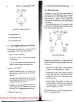
Figure 14.8: Insertion of the point (52,200) followed by splitting of buckets
in Fig. 14.6 lay along the diagonal. Then no matter where
we placed the grid
lines, the buckets off the diagonal would have to be empty.
.
However, if the data is well distributed, and the data file itself is not too
large, then we can choose grid lines so that:
1. There are sufficiently few buckets that
we can keep the bucket matris in
main memory, thus not incurring disk
I/O to consult it, or to add ro~i-s
or columns to the matrix when we introduce
a
new grid line.
2.
We can also keep in memory indexes on the values of the grid lines in
each dimension
(as
per the box "Accessing Buckets of a Grid File"), or
we can avoid the indexes altogether and use main-memory binary
seasch
of the values defining the grid lines in each dimension.
3. The typical bucket does not have more than a few overflow blocks, so
we
do not incur too many disk 1/03 when we search through a bucket.
Under those assumptions, here is
how the grid file behaves on somc important

classes of queries.
Lookup of Specific Points
We are directed to the proper bucket, so the only disk I/O is what is necessary
to read the bucket. If we are inserting or deleting, then an additional disk
write is needed. Inserts that rcquire the creation of an overflow block cause an
additional write.
14.2.
H,ISH-LIKE STRL'CTURES FOR A4ULTIDI~lEhrSIONA4L DATA
681
Partial-Match Queries
Examples of this query
~vould include "find all customers aged 50," or "find all
customers with a salary of
S200K." Sow, ive need to look at all the buckets
in
a row or column of the bucket matrix. The number of disk 110's can be quite
high if there are many buckets in a row or column, but only a small fraction of
all the buckets will be accessed.
Range Queries
A
range query defines a rectangular region of the grid, and all points found
in the buckets that cover that region will be answers to the query, with the
exception of some of the points in buckets on the border of the search region.
For example, if we want to find all customers aged 35-45 with a salary of 50-100,
then we need to look in the four buckets in the lower left of Fig. 14.6. In this
case, all buckets are on the border, so we may look at
a
good number of points
that are not answers to the query. However, if the search region involves a large
number of buckets, then most of them must be interior, and all their points are

answers. For range queries, the number of disk
I/07s may be large, as we may
be required to examine many buckets.
Ho~vever, since range queries tend to
produce large
answer sets, we typically will examine not too many more blocks
than the minimum number of blocks on which the answer could be placed by
any organization
~vhatsoever.
Nearest-Neighbor Queries
Given a point
P,
xve start by searching the bucket in which that point belongs.
If
we find at least one point there. we have a candidate
Q
for the nearest
neighbor. However. it is possible that there are points in adjacent buckets that
are closer to
P
than
Q
is: the situation is like that suggested in Fig. 14.3. We
have to consider n-hether the distance between
P
and
a
border of its bucket is
less than the distance from
P

to
Q.
If there arc such horders, then the adjacent
buckets on the other side of each
such border must be searched also. In fact,
if buckets are severely rectangular
-
much longer in one dimension than the
other
-
then it may be necessary to search even buckets that are not adjacent
to the one containing point
P:
Example
14.10:
Suppose \ve are looking in Fig. 14.6 for the point nearest
P
=
(43,200). We find that (50.120) is the closest point in the bucket, at
a distance of
80.2. So point in the lolver three buckets can be this close to
(4.3.200). because their salary component is at
lnost
90;
so I{-e can omit searching
them. However. the other five buckets must be searched, and lve find that there
are actually
two equally close points: (30.260) and (60,260): at a distance of
61.8 from
P.

Generally, the search for a nearest neighbor can be limited to a
few buckets, and thus a few disk
I/07s.
Horn-ever,
since the buckets nearest the
point
P
may be empty, n-e cannot easily put an upper bound on how costly the
search is.
Please purchase PDF Split-Merge on www.verypdf.com to remove this watermark.
682
CHAPTER
14.
MULTIDIMENSIONAL AND BITMAP INDEXES
14.2.5
Partitioned
Hash Functions
Hash functions can take a list of attribute values as an argument, although
typically they hash values from only one attribute.
For instance, if
a
is an
integer-valued attribute and
b
is a character-string-valued attribute, then we
could add the
value of a to the value of the
ASCII
code for each character of b,
divide by the number of buckets, and take the remainder. The result could be

used as the bucket number of a hash table suitable as
an
index on the pair of
attributes
(a.
b).
.*,
However, such a hash table could only be used in queries that specified
values for both
a
and
b.
A
preferable option is to design the hash function
so it produces some number of bits, say
Ic.
These
k
bits are divided among
n
attributes, so that we produce
ki
bits of the hash value from the ith attribute,
and
C:='=,
ki
=
k.
More precisely, the hash function h is actually a list of hash
functions

(hl,
h2,.
.
. ,
hn), such that
hi
applies to a value for the ith attribute
and produces a sequence of
ki
bits. The bucket in which to place a tuple with
values
(ul,
v2,
.
.
.
,
v,)
for the
n
attributes is computed by concatenating the bit
sequences:
hl (vl)h2(vz)
.
. .
hn(vn).
Example
14.11
:
If we have a hash table with 10-bit bucket numbers (1024

buckets), we could devote four bits to attribute
a
and the remaining six bits to
attribute
b.
Suppose we have a tuple with a-value
A
and b-value
B,
perhaps
with other attributes that are not involved in the hash.
We hash
A
using a
hash function
ha associated with attribute
n
to get four bits, say 0101. n7e
then hash
B,
using a hash function hb, perhaps receiving the six bits 111000.
The bucket number for this tuple is thus 0101111000, the concatenation of the
two bit sequences.
By
partitioning the hash function this way, we get some advantage from
knowing
values for any one or more of the attributes that contribute to the
hash function. For instance, if we are given a value
A
for attribute

a,
and we
find that h,(A)
=
0101, then we know that the only tuples with a-value
d
are in the 64 buckets whose numbers are of the form 0101
.
,
where the
.
.
-
represents any six bits. Similarly, if we axe given the b-value
B
of a tuple. we
can isolate the possible buckets of the tuple to the 16 buckets whose number
ends in the six bits hb(B).
Example
14.12:
Suppose we have the "gold je~velry" data of Example
14.7.
which n-e want to store in a partitioned hash table with eight buckets (i.e three
bits for bucket numbers). We assume as before that two records are all that can
fit in one block.
\Ye shall devote one bit to the age attribute and the remainii~g
two bits to the salary attribute.
For the hash function on age, we shall take the age modulo 2; that is. a
record with an
even age will hash into

a
bucket whose number is of the form
Oxy for some bits x and
y.
A
record a-ith an odd age hashes to one of the buckets
with a number of the form lxy. The hash function for salary
will be the salary
(in thousands) modulo
4.
For example, a salary that leaves a remainder of 1
14.2.
HASH-LIKE STRUCTURES FOR illULTIDIh1ENSIONAL
DATA
683
Figure 14.9:
.4
partitioned hash table
when divided by 4, such as
57K,
will be in a bucket whose number is 201 for
some bit z.
In Fig. 11.9 we see the data from Example 14.7
placed in this hash table.
Sotice that. because we hase used rnostly ages and salaries divisible by 10, the
hash function does not distribute the points too well. Two of the eight buckets
have four records each and need overflow blocks, while three other buckets are
empty.
14.2.6
Comparison

of
Grid Files
and
Partitioned
Hashing
The performance of the ti%-o data structures discussed in this section are quite
different. Here are the major points of comparison.
Partitioned hash tables are actually quite useless for nearest-neighbor
queries
oirange queries. The
is that physical distance between
points is not reflected by the closeness of bucket numbers. Of course
we
could design the hash function on some attribute
a
so the snlallest values
were assigned the first bit string (all O's), the nest values were assigned the
nest hit string
(00
.Dl).
and so on. If we do so, then we have reinvented
the grid file.
A
well chosen hash function will randomize the buckets into which points
fall, and thus buckets will tend
to
be equally occupied. However, grid
files. especially when the number of dimensions is large,
will tend to leave
many buckets

empty or nearly so. The intuitive reason is that when there
Please purchase PDF Split-Merge on www.verypdf.com to remove this watermark.
684
CHAPTER
14.
MULTIDIhPENSIONAL AND
BITMAP
INDEXES
are many attributes, there is likely to be some correlation among at least
some of them, so large regions of the space are left empty. For instance,
we mentioned in Section 14.2.4 that
a
correlation betwen age and salary
would cause most points of Fig.
14.6
to lie near the diagonal, with most of
the rectangle empty.
As
a
consequence, we can use fewer buckets, and/or
have fewer overflow blocks in a partitioned hash table than in a grid file.
Thus, if
we are only required to support partial match queries, where we
specify some attributes' values and leave the other attributes completely un-
specified, then the partitioned hash function is likely to outperform the grid
file. Conversely, if we need to do nearest-neighbor queries or range queries
frequently, then we would prefer to use a grid file.
14.2.7
Exercises for Section
14.2

model
1001
1002
1003
1004
1005
1006
1007
1008
1009
1010
1011
1013
Figure 14.10: Some PC's and their characteristics
Exercise 14.2.1: In Fig. 14.10 are specifications for twelve of the thirteen
PC's introduced in Fig. 5.11. Suppose we wish to design an index on speed and
.
hard-disk size only.
*
a) Choose five grid lines (total for the two dimensions), so that there are no
more than two points in any bucket.
!
b) Can you separate the points with at most two per bucket if you use only
four grid lines? Either show how or argue that it is not possible.
!
c) Suggest
a
partitioned hash function that will partition these points into
four buckets
with at most four points per bucket.

.
Handling
Tiny
Buckets
We generally think of buckets
as
containing about one block's worth of
data. However. there are reasons why we might need to create so many
buckets that
tlie average bucket has only a small fraction of the number
of records that
will fit in a block. For example, high-dimensional data
dl require many buckets if we are to partiti011 significantly along each
dimension. Thus. in the structures of this section and also for the
tree-
based schemes of Section 14.3, rye might choose to pack several buckets
(or nodes of trees) into
one block. If we do so, there arc some i~nportant
points to remember:
The block header must contain information about where each record
is, and to which bucket it belongs.
If we insert a record into
a
bucket, we [nay not have room in the
block containing that bucket. If so,
we need to split the block in
some
way. \Ye must decide which buckets go with each block, find
the records of
each bucket and put them in the proper block, and

adjust the bucket table to point to the proper block.
!
Exercise 14.2.2
:
Suppose we wish to place the data of Fig. 14.10 in a three-
dimensional grid file. based on the speed, ram, and hard-disk attributes. Sug-
gest a partition in
each dimension that will divide the data well.
Exercise 14.2.3: Choose a
hash function
with one bit for each of
the three attributes speed. ram,
and hard-disk that divides the data of Fig. 14.10
1i-eIl.
Exercise 14.2.4: Suppose Ive place the data of Fig. 14.10 in a grid file with
dimensions for speed and ram only. The partitions are at speeds of 720. 950,
1130. and 1350.
and ram of 100 and 200. Suppose also that only two points can
fit in one bucket. Suggest good splits if
~ve insert points at:
*
a)
Speed
=
1000 and ram
=
192.
b)
Speed
=

800. ram
=
128: and thcn speed
=
833, ram
=
96.
Exercise 14.2.5
:
Suppose
IY~
store
a
relati011
R(x.
y)
in a grid file. Both
attributes
have a range of values from 0 to 1000. The partitions of this grid file
happen to be
unifurmly spaced: for
x
there are partitions every 20 units, at 20,
10. GO, and so on. while for
y
the partitions are every 50 units; at 30. 100, 150,
and so on.
Please purchase PDF Split-Merge on www.verypdf.com to remove this watermark.
686
CHAPTER

14.
~~ULTIDIJVIEIVSION-4L AND BITMAP INDEXES
a) How many buckets do
we have to examine to answer the range query
SELECT
*
FROM
R
WHERE
310
<
x
AND
x
<
400
AND
520
<
y
AND
y
<
730;
*!
b) We wish to perform a nearest-neighbor query for the point (110,205).
We begin by searching the bucket with lower-left corner at (100,200) and
upper-right corner at
(120,250), and we find that the closest point in this
bucket is (115,220). What other buckets must be searched to verify that

this point is the closest?
!
Exercise
14.2.6:
Suppose we have a grid file with three lines (i.e., four stripes)
in each dimension. However, the points
(x,
y)
happen to have a special property.
Tell the largest possible number of
nonernpty buckets if:
*
a) The points are on
a
line; i.e., there is are constants a and
b
such that
y
=
ax
+
b
for every point
(x,
y).
b) The points are related quadratically;
i.e., there are constants a,
b,
and
c

such that y
=
ax2
+
bx
+
c
for every point
(x,
y).
Exercise
14.2.7:
Suppose we store a relation R(x, y,
z)
in a partitioned hash
table with 1024 buckets
(i.e., 10-bit bucket addresses). Queries about
R
each
specify exactly one of the attributes, and each of the three attributes is equally
likely to
be
specified. If the hash function produces 5 bits based only on
.r.
3
bits based only on y, and
2
bits based only on
z,
what is the average nuulilber

of buckets that need to be searched to answer
a
query?
!!
Exercise
14.2.8:
Suppose we have
a
hash table whose buckets are numbered
0 to
2"
-
1;
i.e., bucket addresses are
n
bits long. We wish to store in the table
a relation
with two attributes x and
y.
-1
query will either specify a value for
x
or y, but never both. IVith probability
p,
it is x whose value is specified.
a) Suppose we partition the
hash function so that
m
bits are devoted to
x

and the remaining
n
-
m bits to y. As a function of
m,
n,
and
p,
what
is the expected number of buckets that must be examined to answer a
random query?
b) For
I\-hat value of
m
(as a function of
n
and
p)
is the expected number of
buckets minimized? Do not
worry that this
m
is unlikely to be an integer.
*!
Exercise
14.2.9:
Suppose we have a relation R(x,
y)
with 1,000,000 points
randomly distributed. The range of both

z
and
y
is 0 to 1000.
We
can fit 100
tuples of
R
in
a
block. We decide to use a grid file with uniformly spaced grid
lines in each dimension, with
m
as the width of the stripes. we wish to select
rn
in order to minimize the number of disk 110's needed to read all the necessary
pp
7
.
r
-
:-
13.3.
TREE-LIKE STRUCTURES FOR hfULTIDIhfENSIOXAL DATA.
687
buckets to ask
a
range query that is a square 50 units on each side. You
may
assume that the sides of this square

never
align with the grid lines. If we pick
m too large, we shall
have a lot of overflonl blocks in each bucket, and many of
the points in
a
bucket will be outside the range of the query. If we pick m too
small, then there will be too
many
buckets, and blocks will tend not to be full
of data.
What is the best 1-alue of m?
14.3
Tree-Like Structures for Multidimensional
Data
We shall now consider four more structures that are useful for range queries or
nearest-neighbor queries on multidimensional data. In order,
15-e shall consider:
1.
Multiple-key indexes.
2.
kd-trees.
3.
Quad trees.
The first three are intended for sets of points. The R-tree is
comnlonly used to
represent sets of regions: it is also useful for points.
14.3.1
Multiple-Key
Indexes

Suppose we have se~eral attributes representing din~ensio~ls of our data points,
and
we want to support range queries or nearest-neighbor queries on these
points.
-1
simple tree-like scheme for accessing these points is an index of
indexes, or
more generally a tree in which the nodes at each level are indexes
for one attribute.
The idea is suggested in Fig. 14.11 for the case of txvo attributes. The
root of the tree" is an indes for the first of the tw\-o attributes. This index
could be any type of conventional index, such as a B-tree or a hash table. The
index associates with each of its search-key values
-
i.e., values for the first
attribute
-
a pointer to another index.
If
I'
is a value of the first attribute,
then the indes
we
reach bv follov ing key
I'
and its pointer is an index into the
set of
uoints that hare
1.'
for their 1-alue in the first attribute and any value for

the second attribute.
Example
14.13:
Figure 14.12 shows a multiple-key indes for our running
gold jewelry" esample, where the first attribute is age, and the second attribute
is salary. The root
indes. on age, is suggested at the left of Fig. 14.12. We have
not indicated how the index works. For example, the key-pointer pairs forming
the
seven rows of that index might be spread among the leaves of a B-tree.
However, what is important is that the only keys present are
the ages for which
Please purchase PDF Split-Merge on www.verypdf.com to remove this watermark.
688
CHAPTJZR
14.
MULTIDIMENSIONAL AND BITMAP
INDEXES
/k
Index on
first attribute
.
Indexes on
second
attribute
Figure
14.11:
Using nested indexes on different keys
there is one or more data point, and the index makes it easy to find the pointer
associated

with a given key value.
At the right of Fig.
14.12
are seven indexes that provide access to the points
themselves. For example, if we follow the pointer associated
with age
50
in the
root index,
we get to a smaller index where salary is the key, and the four key
values in the index are the four salaries associated with points that have age
50.
Again, we have not indicated in the figure how the index is implemented, just
the key-pointer associations it makes. When we follow the pointers associated
with each of these values
(75,
100, 120,
and
275):
we get to the record for the
individual represented. For instance, following the
pointer
associated
with
100,
we find the person whose age is
50
and whose salary is
$loOK.
In

a
multiple-key index, some of the second or higher rank indexes may be
very small. For example, Fig
14.12
has four second-rank indexes with but a
single pair. Thus, it may be appropriate to implement these indexes
as
simple
tables that are packed several to a block, in the manner suggested by the box
"Handling Tiny Buckets" in Section
14.2.5.
14.3.2
Performance
of
Multiple-Key
Indexes
Let us consider how a multiplr key index performs on various kinds of multidi-
mensional queries.
\I:e shall concentrate on the case of two attributcs, altliough
the generalization to more than two attributes
is
unsurprising.
Partial-Match Queries
If the first attribute is specified. then the access is quite efficient. UTe use the
root index to find the one subindex that leads to the points
n-e want. For
14.3.
TREE-LIKE STRLTCTURES FOR
JIULT1D1.\fERiS10.V~4L
DAZX

689
\=
Figure
14.12:
LIultiple-key indexes for age/salary data
example. if the root is
a
B-tree index, then we shall do two or three disk I/O7s
to
get
to the proper subindex, and then use whatever I/O's are needed to access
all of that index and the points of the data file itself.
On the other hand, if
the first attribute does not have a specified
value; then we must search every
subindex. a potentially time-consuming process.
Range Queries
The multiple-key index works quite well for a range query, prop-ided the indi-
vidual indexes themselves support range queries on their attribute
-
B-trees
or indexed sequential files, for instance. To
answer a range query.
we
use the
root index and the range of the first attribute to find all of the subindexes that
might
contain answer points. \\e then search each of these subindexes. using
the range specified for the
second attribute.

Example
14.14
:
Suppose we have the multiple-key indes of Fig.
14.12
and
i-e are asked the range query
35
5
age
<
55
and
100
5
salary
5
200.
IYhen
ive examine the root indes,
11.c
find that the keys
4.5
and
50
are in
the
range
for age.
\Ve follow the associated pointers to two subindexes on salar~: The

index for age
45
has no salary in the range
100
to
200:
while the index for age
30
has tivo such salaries:
100
and
120.
Thus, the only two points in the range
are
(50.100)
and
(50.120).
0
Please purchase PDF Split-Merge on www.verypdf.com to remove this watermark.
690
CHAPTER
14.
MULTIDIiVfEArSIONAL AXD
BITMAP
lNDEXES
Nearest-Neighbor Queries
The answering of a nearest-neighbor query with a multiple-key index uses the
same strategy
as
for almost

all
the data structures of this chapter. To find the
nearest neighbor of point
(xo, yo), we find a distance d such that we can expect
to find several points within distance
d
of (so, yo). We then ask the range query
xo
-
d
5
2:
5
20
+d
and yo
-
d
5
y
5
yo +d. If there turn out to be no points in
this range, or if there is a point, but distance from
(so, yo) of the closest point
is greater than
d
(and therefore there could be a closer point outside the range,
as
was
discussed in Section

14.1.5),
then we must increase the range and search
again.
However, we can order the search so the closest places are searched first.
A
kd-tree (k-dimensional search tree) is a main-memory data structure gener-
alizing the binary search tree to multidimensional data. We shall present the
idea and then discuss how the idea has been adapted to the block model of
storage.
A
kd-tree is a binary tree in which interior nodes have an associated
attribute a and a value
V
that splits the data points into two parts: those with
a-value less than
V
and those with a-value equal to or greater than
V.
The
attributes at different levels of the tree are different, with levels rotating among
the attributes of all dimensions.
In the classical kd-tree, the data points are placed at the nodes, just
as
in
a binary search tree. However, we shall make two modifications
in our initial
presentation of the idea to take some limited advantage of the block model of
storage.
1.
Interior nodes will have only an attribute, a dividing value for that at-

tribute, and pointers to left and right children.
2.
Leaves will be blocks, with space for as many records as a block can hold.
Example
14.15:
In Fig.
14.13
is a kd-tree for the twelve points of om running
gold-jewelry example.
\&re use blocks that hold only two records for simplicity;
these blocks and their contents are
shorn-n
as square leaves. The interior nodes
are ovals with an attribute
-
either age or salary
-
and a value. For instance,
the root splits by salary, with all records in the left
subtree having a salary less
than
$150K,
and all records in the right subtree having a salary at least
$150I<.
.It the second level, the split is by age. The left child of the root splits at
age
60,
so everything in its left subtree 11-ill have age less than
60
and salary

less than
$l5OK.
Its right subtree will haye age at least
60
and salary less than
Sl5OK.
Figure
14.14
suggests how the various interior nodes split the space
of points into leaf blocks.
For example. the horizontal line at salary
=
1.50
represents the split at the root. The space below that line is split vertically at
age
60,
while the space above is split at age
47,
corresponding to the decision
at the right child of the root.
0
14.3.
TREE-LIKE
STRUCTURES FOR MULTIDII/lENSIONAL DAT-4
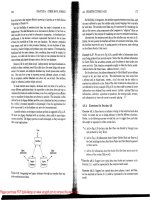
691
Age
38
x
Figure
14.13:

d
kd-tree
14.3.4
Operations
on
kd-Trees
I
lookup of a tuple given values for all dimensions proceeds as in a binary
search tree.
\Ye make a decision which way to go at each interior node and are
directed to a single leaf,
whose block
we
search.
To perform an insertion.
we proceed as for a lookup. \f7e are eventually
directed to a leaf, and if its block has room
we put the new data point there.
If
there is no room, we split the block into two. and we divide its contents
according to whatever attribute is appropriate at the level of the leaf being
split. We create a
new interior node whose children are the two nen- blocks,
and
we install at that interior node a splitting value that is appropriate for the
split
we have just made.'
Example
14.16
:

Suppose someone
35
years old n-ith a salary of
S.50011;
buys
gold
jewelry. Starting at the root, since the salary is at least
$150#
we go to
the right. There.
we colnpare the age
35
with the age
47
at the node. which
directs us to the left. .It the third level. we compare salaries again. and our
salary is greater than
the splitting value.
$300I<.
\Ye are thus directed to a leaf
containing
the points
(25.400)
and
(45.350).
along with the new point
(35.500).
There isn't room for three records in this block, so n-e must split it. The
fourth level splits
on age. so

11-e
havc to pick some age that divides the records
as
evenly as possible. The median value.
3.5.
is a good choice, so we replace the
leaf
by
an interior node that splits on agc
=
35.
To the left of this interior node
is a leaf block with orrly the rccortl
(2.5. -100).
while to the right is a leaf block
with the other t~vo records. as shov-11 in Fig.
14.13.
'One problem that might arise is a situation where there are so many points \vith the same
value in
a
given dimension that tlre hucket
has
only one value in that dimension and cannot
be split. \Ye can try splitting along another
tlirnension. or we can use an a\-erflorv block.
Please purchase PDF Split-Merge on www.verypdf.com to remove this watermark.
692
CHAPTER
14.
hfULTIDIAfEiVSIOIVAL

AND
BITMAP
INDEXES
500K
Salary
Figure 14.14: The partitions implied by the tree of Fig. 14.13
The more complex queries discussed in this chapter are
also supported by a
kd-tree. Here are the key ideas and synopses of the
algorithms:
Partial-Match Queries
If lye are given values for some of the attributes, then we can go one way when
we are at
a
level belonging to an attribute whose value we know. When
we
don't
know the value of the attribute at a node,
we must explore both of its children.
For example, if
we ask for all points with age
=
50 in the tree of Fig. 14.13, we
must look at both children of the root, since the root splits on salary. However.
at the left child of the
root: we need go only to the left, and at the right child
of the root we need only explore its right
subtree. Suppose, for instance, that
the tree
were perfectly balanced, had

a
large number of levels, and had two
dimensions, of which one was specified in the search. Then we would ha~e to
explore both ways at every other level, ultimately reaching about the square
root of the total number of leaves.
Range Queries
Sometimes. a range will allow us to 111uve to only one child of a node, but if
the range straddles the splitting value at the node then
n-e
must explore both
children. For example. given
thc range of ages 35 to
55
and the range of salaries
from
SlOOK to $200K, we would explore the tree of Fig. 14.13
as
follo~vs. The
salary range straddles the $15OK at the root, so we must explore both children.
At
the left child, the range is entirely to the left, so we move to the node with
salary
%OK. Now, the range is entirely to the right, so we reach the leaf with
records (50,100) and
(50.120), both of which meet the range query. Returning
14.3.
TREE-LIKE STRUCTURES
FOR
MULTIDIMENSIONAL
DATA

693
Figure 14.15: Tree after insertion of (35,500)
to the right child of the root, the splitting value age
=
47 tells us to look at both
subtrees.
At the node with salary $300K, we can go only to the left, finding
the point
(30,260), which is actually outside the range.
At
the right child of
the node for age
=
47, we find two other points, both of which are outside the
range.
Nearest-Neighbor Queries
Use the same approach as !.as discussed in Section 14.3.2. Treat the problem
as a range query
with the appropriate range and repeat with
a
larger range if
necessary.
14.3.5
Adapting kd-Trees to Secondary Storage
Suppose we store a file in a kd-tree with
n
leaves. Then the average length
of a path from the root to a leaf
will be about log,
n,

as
for any binary tree.
If we store each node in a block. then as
we traverse a path we must do one
disk
I/O per node. For example, if
n
=
1000, then we shall need about
10
disk
I/O1s, much more than the 2 or 3 disk I/O's that would be typical for a B-tree,
even on a much larger file. In addition. since interior nodes of a kd-tree have
relatively little information, most of the block would be \i,asted space.
We cannot solve the twin problems of long paths and unused space com-
pletely.
Hou-ever. here are two approaches that will make some improvement in
performance.
Multiway Branches at Interior Nodes
Interior nodes of a kd-tree could look more like B-tree nodes, with many key-
pointer pairs. If
we had
n
keys at a node, s-e could split values of an attribute
a
Please purchase PDF Split-Merge on www.verypdf.com to remove this watermark.
694
CHAPTER
14.
MULTIDIA4ENSIONAL AND BITMAP INDEXES

Nothing
Lasts
Forever
Each of the data structures discussed in this chapter allow insertions and
deletions that make local decisions about how to reorganize the structure.
After many database updates, the effects of these local decisions may make
the structure unbalanced in some way. For instance, a grid file may have
too many empty buckets, or a kd-tree may be greatly unbalanced.
It is quite usual for any database to be restructured after a while. By
reloading the database, we have the opportunity to create index structures
that, at least for the moment, are
as
balanced and efficient as is possible
for that type of index. The cost of such restructuring can be amortized
over the large number of updates that led to the imbalance, so the cost
per update is small. However, we do need to be able to "take the database
down";
i.e., make it unavailable for the time it is being reloaded. That
situation may or may not be a problem, depending on the application.
For instance, many databases are taken down overnight, when no one is
accessing them.
into
n
+
1
ranges. If there were
n
+
1
pointers,

we
could follow the appropriate
one to a
subtree that contained only points with attribute
a
in that range.
Problems enter when we try to reorganize nodes, in order to keep distribution
and balance as we do for a B-tree. For example, suppose a node splits on age,
and
we need to merge two of its children, each of which splits on salary. We
cannot simply make one node with all the salary ranges of the two children,
because these ranges will typically overlap. Notice how much easier it
~vould be
if
(as
in a B-tree) the two children both further refined the range of ages.
Group Interior
Nodes
Into Blocks
We may. instead, retain the idea that tree nodes have only
two children. We
could pack many interior nodes into a single block. In order to minimize the
number of blocks that
we must read from disk while traveling down one path,
we are best off including in one block a node and all its descendants for some
number of lerels. That
way, once we retrieve the block with this node, we are
sure to use
some additional nodes on the same block, saving disk 110's. For
instance. suppose

tve can pack three interior nodes into one block. Then in the
tree of Fig.
14.13. n-e ~vould pack the root and its two children into one block.
\Ye could then pack the node for salary
=
80 and its left child into another
block, and we are left
m-ith the node salary
=
300. which belongs on a separate
block; perhaps it could share a block with the latter two nodes, although sharing
requires us to do considerable work when the tree grows or shrinks. Thus, if
we wanted to look up the record (25,60), we n-ould need to traverse only two
blocks, even though we travel through four interior nodes.
14.3.
TREE-LIKE STRUCTURES FOR MULTIDIhfE1YSIONAL DATA
G95
14.3.6
Quad
Trees
In a
quad
tree,
each interior node corresponds to a square region in two di-
mensions, or to a k-dimensional cube in
k
dimensions. As with the other data
structures in this chapter, we shall consider primarily the two-dimensional case.
If the number of points in a square
is

no larger than what will fit in a block,
then we can think of this square as a leaf of the tree, and it is represented by
the block that holds its points. If there are too many points to
fit
in one block,
then
we treat the square as an interior node, with children corresponding to its
four quadrants.
Salary
Figure 14.16: Data organized in a quad tree
Example
14.17:
Figure 14.16 shows the gold-jewelry data points organized
into regions that correspond to nodes of a quad tree. For ease of calculation, we
have restricted the usual space so salary ranges between
0 and $400K, rather
than up to
$5OOK
as in other examples of this chapter. We continue to make
the assumption that only
two records can fit in a block.
Figure 14.17 shows the tree explicitly.
We use the compass designations for
the quadrants and for the children of a node
(e.g., S\V stands for the southm-est
quadrant
-
the points to the left and below the center). 'The order of children
is always as indicated at the root. Each interior node indicates the coordinates
of

the center of its region.
Since the entire space has 12 points, and only
two will
fit
in one block.
we must split the space into quadrants, which we show by the dashed line in
Fig.
14.16. Two of the resulting quadrants
-
the southwest and northeast
-
have only two points. They can be represented by leaves and need not be split
further.
The remaining two quadrants each
have more than two points. Both are split
into subquadrants,
as
suggested by the dotted lines in Fig. 14.16. Each of the
Please purchase PDF Split-Merge on www.verypdf.com to remove this watermark.
696
CHAPTER
14.
IMULTID~~~ENSIO~T,~L
AND
BITMAP
INDEXES
Figure
14.17:
A
quad tree

resulting quadrants has
two or fewer points, so no more splitting is necessary.
0
Since interior nodes of a quad tree in k dimensions have 2%hildren, there
is a range of
k
where nodes fit conveniently into blocks. For instance, if 128, or
27,
pointers can fit in a block, then
k
=
7
is a convenient number of dimensions.
However, for the 2-dimensional case, the situation is not much better than for
kd-trees; an interior node has four children.
Xforeo~-er, while we can choose the
splitting point for a kd-tree node, we are constrained to pick the center of
a
quad-tree region, which may or may not divide the points in that region evenly.
Especially when the
number of dimensions is large, we expect to find many null
pointers (corresponding to empty quadrants) in interior nodes. Of course
we
can be somewhat clever about how high-dimension nodes are represented, and
keep only the non-null pointers and a designation of which quadrant the pointer
represents, thus saving considerable space.
We shall not go into detail regarding the standard operations that we dis-
cussed in Section
14.3.4
for kd-trees. The algorithms for quad trees resenlble

those for kd-trees.
An
R-tree
(region tree) is a data structure that captures some of the spirit of
a
B-tree for multidimensional data. Recall that a B-tree node has a set of keys
that divide a line into segments.
Points along that line belong to only one
segment. as suggested by Fig.
14.18.
The B-tree thus makes it easy for us to
find points; if
we think the point is somewhere along the line represented by
a
B-tree node, we can dcterinine a unique child of that node where the point
could be found.
-
Figure
14.18:
-1
B-tree node divides keys along a line into disjoint segments
14.3.
TREELIKE
STRUCTURES
FOR JlULTIDZ.lIE!VSIO-NAL
DAT.4
697
An R-tree, on the other hand, represents data that consists of 2-dimensional,
or higher-dimensional regions, which we call
data

regzons.
An interior node of
an R-tree corresponds to some
interior
region,
or just "region," which is not
normally a data region. In principle, the region can be
of any shape, although
in practice it is usually a rectangle or other simple shape. The R-tree node
has,
in place of keys, subregions that represent the contents of its children.
Figure
14.19
suggests a node of an R-tree that is associated with the large solid
rectangle. The dotted rectangles represent the subregions associated with four
of its children. Notice that the subregions do not cover the entire region, which
is satisfactory
as
long as all the data regions that lie within the large region are
wholly contained within one of the small regions. Further, the subregions are
allowed to overlap, although it is desirable to keep the overlap small.
Figure
14.19:
The region of an R-tree node and subregions of its children
14.3.8
Operations
on
R-trees
A
typical query for tvhich an R-tree is useful is

a
"~vhere-am-Z" query, \vhich
specifies
a
point
P
and asks for the data region or regions
in
which the point lies.
i7e start at the root, with which the entire region is associated. We examine
the subregions at the root and determine which children of the root correspond
to interior
regions that contain point
P.
Note that there may be zero, one, or
several such regions.
If there are zero regions, then we are done;
P
is not in any data region. If
there is at least one interior region that contains
P,
then 11-e must recursively
search for
P
at the child corresponding to
each
such region. IVhen we reach
one or more leaves,
XI-e shall find the actual data regions, along with either the
complete record for each data region or a pointer to that record.

When we insert a neK region
R
into an R-tree. we start at the root and try
to find a subregion into n-hich
R
fits. If there is more than one such region. then
we pick one: go to its corresponding child, and repeat the process there. If
there
is no subregion that contains
R,
then
we
have to expand one of the subregions.
"
Ii'hich one to pick may be a difficult decision. Intuitively. we want to espand
regions
as
little as possible. so we might ask which of the children's subregions
would have their area increased
as
little as possible, change the boundary of
that region to include
R.
and recursively insert
R
at the corresponding child.
Please purchase PDF Split-Merge on www.verypdf.com to remove this watermark.
698
CHAPTER
14.

AIULTIDIJENSIONAL
AND
BIThIAP INDEXES
Eventually. we reach a leaf, where we insert the region
R.
However, if there
is no room for
R
at that leaf, then me must split the leaf. How we split the
leaf is subject to some choice. We generally want the two subregions to be
as
small
as
possible, yet they must, between them, cover all the data regions of
the original leaf. Having split the leaf, we replace the region and pointer for the
original leaf at the node above by a pair of regions and pointers corresponding
to the two new leaves. If there is room at the parent, we are done. Otherwise,
as
in a B-tree, we recursively split nodes going up the tree.
Figure 14.20: Splitting the set
of
objects
Example
14.18:
Let us consider the addition of a new region to the map of
Fig.
14.1. Suppose that leaves have room for six regions. Further suppose that
the six regions of Fig. 14.1 are together on one leaf, whose region is represented
by
the outer (solid) rectangle

in
Fig. 11.20.
Kow, suppose the local cellular phone company adds a
POP
(point of pres-
ence) at the position shown in Fig. 14.20. Since the seven data regions do not fit
on one leaf,
we shall split the leaf. with four in one leaf and three in the other.
Our options are man)-: n-e have picked in Fig. 14.20 the division (indicated
by
the inner, dashed rectangles) that minimizes the overlap, ~vl~ile splitting the
leaves as evenly
as
possible.
\Ye show in Fig. 14.21 hotv the tn-o new leaves fit into the R-tree. The parent
of these nodes has pointers to both leaves, and associated with the pointers are
the
lo&er-left and upper-right corners of the rectangular regions covered by each
leaf.
0
Example
14.19
:
Suppose we inserted another house below house2, with lower-
left
coordinates (70,s) and upper-right coordinates
(80,15).
Since this house is
14.3.
TREE-LIKE STRUCTURES

FOR
hlULTIDIAIE.NSIONAL DATA
699
3
%"<
/
Figure 14.21: An R-tree
lM
m
Figure 14.22: Extending a region to accommodate new data
not wholly contained
mithin either of the leaves' regions, we must choose which
region to
espand. If we expand the lo~ver subregion, corresponding to the first
leaf in Fig. 14.21, then
we add 1000 square units to the region, since we extend
it 20 units to
the right. If we extend the other subregion
by
lowering its bottom
by 15 units, then we add 1200 square units. We prefer the first, and the new
regions are changed in Fig. 14.22.
\Ye also must change the description of the
region
0
in the top node of Fig. 14.21 from ((0,O). (60,50)) to ((O,O), (@,so)).
14.3.9
Exercises
for
Section

14.3
Exercise
14.3.1:
Shov; a multiple-key index for the data of Fig. 14.10 if the
indexes are on:
Please purchase PDF Split-Merge on www.verypdf.com to remove this watermark.
700
CHAPTER
14.
MULTIDIMENSIONAL
AND
BITMAP INDEXES
a) Speed, then ram.
b) Ram then hard-disk.
c) Speed, then ram, then hard-disk.
Exercise
14.3.2
:
Place the data of Fig. 14.10 in a kd-tree. Assume two records
can fit in one block. At each level, pick a separating value that divides the data
as
evenly
as
possible. For an order of the splitting attributes choose:
a) Speed, then ram, alternating.
b) Speed, then ram, then hard-disk, alternating.
c)
Whatever attribute produces the most even split at each node.
Exercise
14.3.3:

Suppose we have a relation
R(x,y,
z),
where the pair of
attributes
x
and
y
together form the key. Attribute
x
ranges from
1
to 100,
and
y
ranges from
1
to 1000. For each
x
there are records with 100 different
values of
y,
and for each
y
there are records with 10 different values of
x.
Xote
that there are thus 10,000 records in
R.
We wish to use a multiple-key index

that will help us to answer queries of the form
SELECT
z
FROM
R
WHERE
x
=
C
AND
y
=
D;
where
C
and
D
are constants. Assume that blocks can hold ten key-pointer
pairs, and we wish to create dense indexes at each level, perhaps with sparse
higher-level indexes above them, so that each index starts from a single block.
Also assume that initially all index and data blocks are on disk.
*
a) How many disk I/O's are necessary to answer a query of the above form
if the first index is on
x?
b)
How many disk
1/03
are necessary to answer a query of the above form
if the first index is on

y?
!
c) Suppose you were allowed to buffer
11
blocks in memory
at
all times.
Which blocks
would you choose, and would you make
x
or
y
the first
index, if you wanted to minimize the
number of additional disk I/O's
needed?
Exercise
14.3.4:
For the structure of Exercise 11.3.3(a), how many disk I/O's
are required to answer the range query in which 20
5
x
5
35 and 200
5
y
5
350.
.issume data is distributed uniformly; i.e., the expected number of points will
be found within any given range.

Exercise
14.3.5
:
In the tree of Fig. 14.13, what new points would be directed
to:
14.3.
TREE-LIKE STRUCTURES
FOR
MZiLTIDIAlENSIONAL DtLT.4
701
*
a) The block with point (30,260)?
b) The block with points (50,100) and (50,120)?
Exercise
14.3.6:
Show a possible evolution of the tree of Fig. 14.15 if we
insert the points (20,110) and then (40,400).
!
Exercise
14.3.7:
We mentioned that if a kd-tree were perfectly balanced, and
we execute a partial-match query in which one of
two attributes has a value
specified, then vie wind up looking at about
fi
out of the
n
leaves.
a) Explain why.
b) If the tree split alternately in d dimensions, and

we specified values for
m
of those dimensions, what fraction of the leaves
we expect to have
to search?
c)
How does the performance of (b) compare with a partitioned hash table?
Exercise
14.3.8
:
Place the data of Fig. 14.10 in a quad tree with dimensions
speed and ram. Assume the range for speed is 100 to 300, and for ram it is
0
to 256.
Exercise
14.3.9:
Repeat Exercise 14.3.8 with the addition of a third dimen-
sion, hard-disk, that ranges from 0 to 32.
*!
Exercise
14.3.10
:
If 1-e are allos-ed to put the central point in a quadrant of a
quad tree
wherever I\-e nant, can .se always divide a quadrant into subquadrants
with an equal number of points (or
as
equal
as
possible, if the number of points

in the quadrant is not divisible by
4)?
Justify your answer.
!
Exercise
14.3.11:
Suppose 1-e ha~e a database of 1.000,000 regions, which
may overlap.
Xodes (blocks) of an R-tree can hold 100 regions and pointers.
The region represented by any node has 100 subregions. and the
o~erlap among
these regions is such that the total area of the 100 subregions is 130% of the
area of the region. If
we perform a .'I\-here-am-I" query for a giren point. how
many blocks do we expect to retrieve?
!
Exercise
14.3.12
:
In the R-tree represented by Fig. 1-1.22, a ne\v region might
go into the subregion containing the school or the subregion containing housed.
Describe the rectangular regions for which we
~sould prefer to place the new
region in the subregion
with the school (i.e., that choice minimizes the increase
in the subregion size).
Please purchase PDF Split-Merge on www.verypdf.com to remove this watermark.
702
CHAPTER
14.

AlULTIDIMENSIONAL AND BITMAP INDEXES
14.4.
BITlUAP INDEXES
14.4
Bitmap
Indexes
Let us now turn to a type of index that is rather different from the kinds seen
so
far. M'e begin by imagining that records of
a
file have permanent numbers,
1,2,
.
. .
,
n.
hloreover, there is some data structure for the file that lets us find
the ith record easily for any
i.
A
bitmap
index
for a field
F
is a collection of bit-vectors of length
n,
one
for each possible value that may appear in the field
F.
The vector for iralue

u
has
1
in position
i
if the ith record has
v
in field
F,
and it
ha5
0 there if not.
Example
14.20
:
Suppose a file consists of records with two fields,
F
and
G,
of
type integer and string, respectively. The current file has six records, numbered
1
through
6,
with the following values in order: (30,
f
oo), (30, bar), (40, baz),
(50,
f
oo), (40, bar), (30, baz).

A
bitmap index for the first field,
F,
would have three bit-vectors, each of
length
6.
The first, for value 30, is 110001, because the first, second, and sixth
records have
F
=
30. The other two, for 40 and 50, respectively, are 001010
and
000100.
A
bitmap index for
G
would also have three bit-vectors, because there are
three different strings appearing there. The three bit-vectors are:
Value
I
Vector
foo
I
100100
In each case, the 1's indicate in which records the corresponding string appears.
0
14.4.1
Motivation
for
Bitmap

Indexes
It might at first appear that bitmap indexes require much too much space,
especially when there are many different values for a field, since the total number
of bits is
the product of the number of records and the number of values. For
example, if the field is a key, and there are
n
records, then
n2
bits are used
among all the bit-vectors for that field. However, compression can be used to
make the number of bits closer to
n,
independent of the number of different
~alues,
as
we shall see in Section 14.4.2.
You might also suspect that there are problems managing the bitmap
in-
dexes. For example, they depend on the number of a record remaining the same
throughout time.
How do we find the ith record as the file adds and deletes
records? Similarly, values for a field
may appear or disappear. How do we find
the bitmap for a value efficiently? These and related questions are discussed in
Section 14.4.4.
The compensating advantage of
bitmap indexes is that they allow us to
answer partial-match queries very efficiently in many situations. In a sense they
offer the advantages of buckets that we discussed in Example 13.16, where

\ve
found the Movie tuples with specified values in several attributes without first
retrieving all the records that matched in each of the attributes. An example
will illustrate the point.
Example
14.21
:
Recall Example 13.16, where we queried the Movie relation
with the query
SELECT
title
FROM Movie
WHERE
studioName
=
'Disney'
AND
year
=
1995;
Suppose there are bitmap indexes on both attributes studioName and year.
Then we can intersect the vectors for year
=
1995 and studioName
=
'Disney';
that is, we take the
bitwise
AND
of these vectors, which will give us a vector

with a
1
in position
i
if and only if the ith Movie tuple is for a movie made by
Disney in 1995.
If we can retrieve tuples of Movie given their numbers, then
I\-e Aeed to
read only those blocks containing one or more of these tuples, just
as
n*e did in
Example 13.16. To intersect the bit vectors, we must read them
into memory,
which requires a disk
I/O
for each block occupied by one of the two vectors. As
mentioned, we shall
later address both matters: accessing records given their
numbers in Section 14.4.4 and making sure the bit-vectors do not occupy too
much space in Section 14.4.2.
Bitmap indexes can also help answer range queries. We shall consider an
example next that
both illustrates their use for range queries and
shorn-s
in detail
with short bit-vectors how the bitwise
ASD
and
OR
of bit-vectors can be used

to discover the
answer to a query without looking at any records but the ones
me want.
Example
14.22:
Consider the gold jelvelry data first introduced in Exam-
ple 14.7. Suppose that the twelve points of that example are records numbered
from
1
to 12 as follo~us:
For the first component, age, there are seven different values: so the bitmap
index for age consists of the follo\ving seven vectors:
25: 100000001000
30:
000000010000
45:
010000000100
50:
0011
1OOOOOlO
60: 000000000001
TO:
000001000000
85: 000000100000
For the salary component, there are ten different values, so the salary
bitmap
index has the following ten bit-vectors:
Please purchase PDF Split-Merge on www.verypdf.com to remove this watermark.
704
CHAPTER

14.
~~ULTIDI~V~ENSIONAL
AhTD
BITAJAP
INDEXES
GO: 110000000000 75: 001000000000 100: 000100000000
110: 000001000000 120: 000010000000 140: 000000100000
260:
000000010001 275: 000000000010 350: 000000000100
400: 000000001000
Suppose we want to find the jewelry buyers with an age in the range 45-55
and a salary in the range 100-200.
We first find the bit-vectors for the age
values
in
this range; in this example there are only two: 010000000100 and
001110000010, for 45 and 50, respectively. If
we
take their bitwise OR, we have
a new bit-vector with
1
in position
i
if and only if the ith record has an age in
the desired range. This bit-vector is 011110000110.
Next, we find the bit-vectors for the salaries between 100 and 200 thousand.
There are four, corresponding to salaries 100, 110, 120, and 140; their
bitwise
OR is 000111100000.
The last step is to take the

bitwise
AND
of the two bit-vectors we calculated
by OR. That is:
011110000110
AND
000111100000
=
000110000000
\Ve thus find that only the fourth and fifth records, which are (50,100) and
(50,120), are in the desired range.
14.4.2
Compressed Bitmaps
Suppose we have a bitmap index on field
F
of a file with
n
records, and there
are
m
different values for field
F
that appear in the file. Then the number of
bits in all the bit-vectors for this index is
mn.
If, say, blocks are 4096 bytes
long, then we can fit 32,768 bits in one block, so the number of blocks needed
is
mn/32768. That number can be small compared to the number of blocks
needed to hold the file itself, but the larger

m
is, the more space the bitmap
index takes.
But if m is large, then
1's in a bit-vector will be very rare; precisely, the
probability that any bit is
1
is llm. If 1's are rare, then we have an opportunity
to encode bit-vectors so that they take much
fewer than
n
bits on the average.
-4
comrnon approach is called
run-length encoding.
where ~ve represent a
run,
that is, a sequence of
i
0's followed by a 1, by some suitable binary encoding
of the integer
i.
\Ve concatenate the codes for each run together, and that
sequence of bits is the encoding of the entire bit-vector.
\Ye might imagine that we could just represent integer
i
by expressing
i
as
a

binary number. However, that simple a scheme will not do, because it
is not possible to break a sequence of codes apart to determine uniquely the
lengths of the runs involved (see the box on "Binary Numbers
Won't Serve as a
Run-Length Encoding"). Thus,
the encoding of i~~tegers
i
that represent a run
length must be more complex than a simple binary representation.
We
shall study one of many possible schemes for
encoding.
There are some
better, more complex schemes that can improve on the amount of compression
Binary Numbers Won't Serve as a Run-Length
Encoding
Suppose we represented a run of i 0's followed by a
1
with the integer
i
in
binary. Then the bit-vector
000101 consists of two runs, of lengths 3 and 1,
respectively. The binary representations of these integers are 11
and 1, so
the run-length encoding of
000101 is
111.
However, a similar calculation
shows that the bit-vector

010001 is also encoded by 111; bit-vector 010101
is a third vector encoded by
111.
Thus,
111
cannot be decoded uniquely
into one bit-vector.
achieved here, by almost a factor of 2, but only when typical runs are very long.
In our scheme,
we first determine how many bits the binary representation of
i
has. This number
j,
which is approximately log,
i,
is represented
in
"unary,"
by
j
-
1 1's and a single 0. Then, we can follow with
i
in binary.*
Example
14.23: If
i
=
13, then
j

=
4; that is, we need 4 bits in the binary
representation of
i.
Thus. the encoding for
i
begins with 1110. We follow with
i
in binary, or 1101. Thus, the encoding for 13 is 11101101.
The encoding for
i
=
1
is 01; and the encoding for
i
=
0 is 00. In each
case,
j
=
1, so we begin with a single 0 and follow that 0 with the one bit that
represents
i.
If we concatenate a sequence of integer codes, \ye can al~vaq-s recover the
sequence of run lengths and therefore recover the original bit-vector. Suppose
we have scanned some of the encoded bits, and
we are now at the beginning
of a sequence of bits that encodes some integer
i.
We scan forward to the first

0, to determine the value of
j.
That is,
j
equals the number of bits we must
scan until we get to the first 0 (including that 0 in the count of bits). Once we
know
j.
we look at the next
j
bits;
i
is the integer represented there in binary.
lloreover, once
13-e
have scanned the bits representing
i.
we know ~vhere the
next code for an integer begins. so
1-e
can repeat the process.
Example
14.24: Let us decode thc sequence 11101101001011. Starting at the
beginning.
tve find the first 0 at the 4th bit. so
j
=
4. The next
1
bits are 1101.

so
we determine that the first integer is 13. \Ye are no\\- left wit11 001011 to
decode.
Since the first bit is
0: we know thc nest bit represents the next integer by
itself: this integer is
0. Thus, we have decoded the sequence 13, 0, and
must
decode the remaining sequence 1011.
2Actually. except for the case that
j
=
1
(i.e
i
=
0
or
i
=
I),
we can be sure that the
binary representation
of
i
begins with
1.
Thus, \re can save about one bit per number
if
we

omit this
1
and use only the remaining
j
-
1 bits.
Please purchase PDF Split-Merge on www.verypdf.com to remove this watermark.
706
CHAPTER
14.
IMULTIDI~MENSIONA
L
AXD
BIThfA
P
INDEXES
\Ve find the first 0 in the second position, whereupon we conclude that the
final two bits represent the last integer,
3.
Our entire sequence of run-lengths
is thus 13, 0,
3.
From
these numbers, we can reconstruct the actual bit-vector,
00000000000001 10001.
Technically, every bit-vector so decoded will end in
a
1, and any trailing 0's
will not be recovered. Since we presumably know the number of records in the
file, the additional

0's can be added. However, since 0 in a bit-vector indicates
the corresponding record is not in the described set, we don't even have to know
the total number of records, and can ignore the trailing
0's.
Example
14.25:
Let us convert some of the bit-vectors from Example 14.23
to our run-length code. The vectors for the first three ages, 25, 30, and 45,
are 100000001000,000000010000, and 010000000100, respectively. The first of
these has the run-length sequence
(0,7).
The code for 0 is 00, and the code for
'7
is 110111. Thus, the bit-vector for age 25 becomes 00110111.
Similarly, the bit-vector for age 30 has only one run, with seven
0's. Thus,
its code is 110111. The bit-vector for age 45 has
two runs, (1,7). Since
1
has
the code 01, and we determined that
7
has the code 110111, the code for the
third bit-vector is 01110111.
U
The compression in Example 14.25 is not great. However, we cannot see the
true benefits when
n, the number of records, is small. To appreciate the value
of the encoding, suppose that
m

=
n, i.e., each ~alue for the field on which the
bitmap index is constructed, has a unique value. Xotice that the code for a run
of length
i
has about 210ga
i
bits. If each bit-vector has a single 1, then it has
a single run, and the length of that run cannot
be
longer than n. Thus, 2 log,
n
bits is
an
upper bound on the length of a bit-vector's code in this case.
Since there are
n
bit-vectors in the index (because
m
=
n),
the total number
of hits to represent the index is at most
2nlog2
la.
Notice that without the
encoding,
nQits would be required.
.4s
long as

n
>
4, we have
211
loga n
<
n'.
and as
YZ
grows,
271.
log2
n
becomes arbitrarily sinaller than na.
14.4.3
Operating on Run-Length-Encoded Bit-Vectors
\\-hen we need to perform bitwise
AND
or
OR
on encoded bit-vectors, ive
ha~e little choice but to decode them and operate on the original bit-vectors.
However,
we do not have to do the decoding all at once. The compression
scheme
1-e
have described lets us decode one run at a time, and \ve can thus
determine wl~ere the nest I is in each operand bit-vector. If we are taking the
OR.
we can produce a

1
at that position of the output, and if we arc taking the
i?;D
we produce a
1
if
and
only if both operands have their next 1 at the sanlc
position. The algorithms involved are comples. but an example ma>- ~nakc the
idea adequately clear.
Example
14.26
:
Consider the encoded bit-vectors we obtained in Exam-
ple
14.25 for ages 25 and 30: 00110111 and 110111, respectively. We can decode
14.4.
BIT-VfiP
INDEXES
their first runs easily; we find they are 0 and
7,
respectixrely. That is, the first
1
of the bit-vector for
25
occurs in position 1, while the first
1
in the bit-vector
for
30

occurs at position
8.
We therefore generate
1
in position
1.
Next, we must decode the next run for age 25, since that bit-vector may
produce another
1
before age 30's bit-vector produces a
1
at position
8.
How-
ever, the next run for age 25 is 7, which says that this bit-vector next produces
a
1
at position
9.
?\'e therefore generate six 0's and the
1
at position
8
that
comes from the bit-vector for age
30. Xow, that bit-vector contributes no more
1's to the output. The 1 at position
9
from age 25's bit-vector is produced, and
that bit-vector too produces no subsequent

1's.
\Ve conclude that the
OR
of these bit-vectors is 100000011. Referring to
the original
bit-vectors of length 12, we see that is almost right; there are three
trailing
0's omitted. If we know that the number of records in the file is 12, we
can append those
0's. However, it doesn't matter whether or not we append
the
O's, since only a
1
can cause
a
record to be retrieved. In this example, we
shall not retrieve any of records 10 through 12 anyway.
0
14.4.4
Managing Bitmap Indexes
We have described operations on bitmap indexes without addressing three im-
portant issues:
1. When we want to find the bit-vector for
a
given value, or the bit-vectors
corresponding to values in
a
given range, how do we find these efficiently?
2. When
we have selected a set of records that answer our query, how do rvc

retrieve those records efficiently?
3.
TVhen the data file changes by insertion or deletion of records. how do we
adjust the
bitmap index on
a
given field?
Finding
Bit-Vectors
The first question can be answered based on techniques
we have already learned.
Think of each bit-rector
as
a record whose key is the value corresponding to this
bit-vector (although the value itself does not appear in this "record"). Then
any secondary index technique
will take us efficiently from values to their bit-
vectors. For exanlple, we could use a B-tree, whose leaves contain key-pointer
pairs; the pointer leads to the bit-vector for the key value. The B-tree is often
a
good choice, because it supports range queries easily, but hash tables or
indexed-sequential files are other options.
We also need to store the bit-vectors somewhere. It is best to think of
them as variable-length records. since they
ill
generally grow
as
more records
are added to the data file. If the bit-vectors, perhaps in compressed
form.

are typically shorter than blocks. then n-e can consider packing several to a
block and moving them around
as
needed. If bit-vectors are typically longer
Please purchase PDF Split-Merge on www.verypdf.com to remove this watermark.
708
CHAPTER
14.
MULTIDIh.IENSIOArAL AND BITMAP INDEXES
than blocks, we should consider using a chain of blocks to hold each one. The
techniques of Section
12.4
are useful.
Finding
Records
Sow let us consider the second question: once
we have determined that we need
record
k
of the data file, how do we find it. Again, techniques we have seen
already may be adapted. Think of the
kth record as having search-key value
k
(although this key does not actually appear in the record). We may then
create
a
secondary index on the data file, whose search key is the number of
the record.
If there is no reason to organize the file
any

other way, we can even use
the record number as the search key for a primary index,
as
discussed in Sec-
tion
13.1.
Then, the file organization is particularly simple, since record num-
bers never change (even
as
records are deleted), and we only have to add new
records to the end of the data file.
It
is thus possible to pack blocks of the data
file completely full, instead of leaving extra space for insertions into the middle
of the file
as
we found necessary for the general case of
an
indexed-sequential
file
in Section
13.1.6.
Handling Modifications
to
the Data File
There are
two aspects to the problem of reflecting data-file modifications in
a
bitmap index.
1.

Record numbers must remain fised once assigned.
2.
Changes to the data file require the bitmap index to change as well.
The consequence of point
(1)
is that \\.hen we delete record
i,
it is easiest
to "retire" its number. Its space is replaced by a "tombstone" in the data file.
The
bitmap index must also be changed, since the bit-vector that had a
1
in
position
i
must have that
1
changed to
0.
Sate that we can find the appropriate
bit-vector, since we know what value record
i
had before deletion.
Next consider insertion of a new record. We keep track of the next available
record number and assign it to the new record. Then, for each
bitmap index.
KT
must determine the value the new record has in the corresponding field and
modify the bit-rector for that value
by

appendine a
1
at the end. Technicallv,
"
all
the other bit-vectors in this indes get a new
0
at the end, but if \re arc using
a
con~pression technique such as that of Section
14.1.2.
then no change to the
comprrssed values is ncedcd.
hs a special case, the new record may hare
a
value for thc indexed field
that has not been seen before. In that case, we need a new bit-vector for
this value, and this bit-vector and its corresponding value need to be inserted
into the secondary-index structure that is used to
find a bit-vector given its
corresponding
value.
14.4.
BITX4.4
P INDEXES
Last, let us consider a modification to a record
i
of the data file that changes
the value of
a

field that has a bitmap index, say from value
v
to vdue
w.
We
must find the bit-vector for
v
and change the
1
in position
i
to
0.
If there is
a
bit-vector for value
w,
then n-e change its
0
in position
i
to
1.
If there is not
yet
a
bit-vector for
w,
then we create it
as

discussed in the paragraph above for
the case when an insertion introduces a new value.
14.4.5
Exercises
for
Section
14.4
Exercise
14.4.1
:
For the data
of
Fig.
14.10
show the bitmap indexes for the
attributes:
*
a) Speed,
b) Ram, and
both in
(i)
uncompressed form, and
(ii)
compressed form using the scheme of
Section
14.4.2.
Exercise
14.4.2
:
Using the bitmaps of Example

14.22,
find the jewelry buyers
with an age in the range
20-40
and
a salary in the range
0-100.
Exercise
14.4.3
:
Consider a file of
1,000,000
records, with a field
F
that has
m
different values.
a)
As a function of
m.
hol~ many bytes does the bitnlap index for
F
have?
!
b)
Suppose that the records numbered from
1
to
1,000,000
are given values

for the field
F
in a round-robin fashion, so each value appears cvery
in
records. How many bytes would be consumed by
a
compressed index?
!!
Exercise
14.4.4
:
\Ve suggested in Section
14.4.2
that it
was
possible to reduce
the number of bits taken to encode number
i
from the
2
log,
i
that we used in
that section until
it
is close to logz
i.
Show how to approach that limit
as
closely

as
you like, as long as
i
is large.
Hint:
We used a unary encoding of the length
of the binary encoding that
we used for
i.
Can you encode the length of the
code in binary?
Exercise
14.4.5:
Encode, using the scheme of Section
14.4.2.
the follo\ving
bitn~aps:
Please purchase PDF Split-Merge on www.verypdf.com to remove this watermark.
710
CHAPTER
14.
MULTIDI.kIENSI0NAL AND BITMAP INDEXES
*!
Exercise 14.4.6: Itre pointed out that compressed bitmap indexes consume
about
2n
log,
n
bits for a file of
n

records. HOW does this number of bits compare
with the number of bits consumed by a B-tree index? Remember that the
B-
tree index's size depends on the size of keys and pointers, as well as (to a small
extent) on the size of blocks. However, make some reasonable estimates of these
parameters in your calculations. Why might we prefer a B-tree, even if it takes
more space than compressed bitmaps?
14.5
Summary
of
Chapter
14
+
Multidimensional Data:
Many applications, such as geographic databases
or sales and inventory data, can be thought of
as
points in a space of two
or more dimensions.
+
Queries Needing Multidimensional Indexes:
The sorts of queries that
need to be supported on multidimensional data include partial-match (all
points with specified values in a subset of the dimensions), range queries
(all points within a range in each dimension), nearest-neighbor (closest
point to a given point), and where-am-i (region or regions containing a
given point).
+
Executing Nearest-Neighbor Queries:
.\iany

data structures allow nearest-
neighbor queries to be executed by performing a range query around the
target point, and expanding the range if there is no point in that range.
\Ire must be careful, because finding a point within a rectangular range
may not rule out the possibility of a closer point outside that rectangle.
+
Grid Files:
The grid file slices the space of points in each of the dimen-
sions. The grid lines can be spaced differently, and there can be different
numbers of lines for each dimension. Grid files support
range queries,
partial-match queries, and nearest-neighbor queries
\%-ell, as long
as
data
is fairly uniform in distribution.'
+
Partitioned Hash Tables:
.4
partitioned hash function constructs some
bits of the bucket number
from each dimension. They support partial-
match queries
well, and are not dependent on thc data being uniformly
distributed.
+
Multiple-Key Indexes:
.A
simple ~tiultidimensional structure has
a

root
that is an index on one attribute. leading to a collection of indescs on a
second attribute, which can lead to indexes on
a
third attribute, and
so
on. They are useful for range and nearest-neighbor queries.
+
kd-Trees:
These trees are like binary search trees: but t,hey branch on
different attributes at different
lerels. They support partial-~natch, range,
and nearest-neighbor queries well. Some careful packing of tree nodes into
14.6.
REFEREXCES
FOR
CHAPTER
14
711
blocks must be done to make the structure suitable for secondary-storage
operations.
+
Quad Pees:
The quad tree divides a multidimensional cube into quad-
rants, and recursively divides the quadrants the same way if they
have too
many points. They support partial-match, range, and nearest-neighbor
queries.
+
R-Bees:

This form of tree normally represents a collection of regions by
grouping them into a hierarchy of larger regions. It helps with where-am-
i queries and, if the atomic regions are actually points, will support the
other types of queries studied in this chapter,
as
well.
+
Bitmap Indexes:
Multidimensional queries are supported by a form of
index that orders the points or records and represents the positions of the
records with a given
value in an attribute by a bit vector. These indexes
support range, nearest-neighbor, and partial-match queries.
+
Compressed Bitmaps:
In order to save space, the bitmap indexes, which
tend to consist of vectors with very few
l's, are compressed by using a
run-length encoding.
14.6
References
for
Chapter
14
Most of the data structures discussed in this section were the product of research
in the
1970's
or early 1980's. The kd-tree is from [2]. Modifications suitable
for secondary storage appeared in [3] and
[13]. Partitioned hashing and its use

in partial-match
retieval is from [I21 and
131.
However. the design idea from
Exercise 14.2.8 is
from
[14].
Grid files first appeared in
[9]
and the quad tree in [6]. The R-tree is from
[8], and two extensions [Is] and [I] are ~vell known.
The
bitmap index has an interesting history. There
was
a company called
Nucleus, founded by Ted
Glaser, that patented the idea and developed a
DBMS
in which the bitmap index was both the index structure and the data repre-
sentation. The company failed in the late
1980's, but the idea has recently
been incorporated into several major commercial database systems. The first
published
xork on the subject
was
[lo]. [Ill is a recent expansion of the idea.
There are a number of surreys of multidimensional storage structures. One
of the earliest is
[4].
More recent surveys are found in [16] and [i]. The former

also includes surveys of
several other important database topics.
1.
X.
Beckn~ann: H P. Icriegel,
R.
Schneider, and
B.
Seeger. "The R*-tree:
an
efficient and robust access method for points and rectangles,"
Proc.
ACM
SIGMOD
Intl. Conf. on Management of Data
(1990), pp. 322-331.
2.
J.
L.
Bentley, "~Iultidimensional binary search trees used for associative
searching."
Comm. ACM
18:9 (1975), pp. 509-517.
Please purchase PDF Split-Merge on www.verypdf.com to remove this watermark.
712
CHAPTER
14.
MULTIDIL;MENSIONAL AND BITSiAP IArDEXES
3.
J.

L.
Bentley, "Multidimensional binary search trees in database applica-
tions,"
IEEE
lkans. on Software Engineering
SE-5:4(1979), pp. 333-310.
4.
J.
L.
Bentley and
J.
H.
Friedman, "Data structures for range searching,"
Computing Surueys
13:3
(1979), pp. 397-409.
t
5.
W.
A.
Burkhard, "Hashing and trie algorithms for partial match re-
trievaI,"
ACM Buns. on Database Systems
1:2 (1976), p~. 175-187.
Chapter
15
6.
R.
A.
Finkel and

J.
L. Bentley, "Quad trees, a data structure for retrieval
1
on composite keys,"
Acta
Informatics
4:l
(1974), pp. 1-9.
7.
V.
Gaede and
0.
Gunther, "Multidimensional access methods,"
cornput-
Query
Execution
ing Surveys
30:2 (1998), pp. 170-231.
8.
A.
Guttman, "R-trees: a dynamic index structure for spatial searching,"
Proc. ACM SIGMOD Intl. Conf. on Management of Data
(1984), pp. 47-
r
w
9.
J.
Nievergelt,
H.
Hinterberger, and

I<.
Sevcik, "The grid file:
an
adaptable,
symmetric, multikey file structure,"
ACM Trans. on Database Systems
9:l
(1984), pp. 38-71.
10.
P.
O'Xeil, "Model 204 architecture and performance,"
Proc. Second Intl.
Workshop on
High
Performance Transaction Systems,
Springer-Verlag,
Berlin, 1987.
11.
P.
O'Neil and D. Quass, "Improved query performance with variant in-
dexes,"
Proc. ACM SIGMOD Intl. Conf. on Management of Data
(1997),
pp. 38-49.
12.
R.
L.
Rivest, "Partial match retrieval algorithms,"
SIAM
J.

Computing
5:l (1976), pp. 19-50.
13.
J.
T.
Robinson, "The K-D-B-tree: a search structure for large multidi-
mensional dynamic indexes,"
Proc. ACM SIGMOD Intl. Conf. on Mam-
agement of Data
(1981): pp. 10-18.
14.
J.
B. Rothnie Jr. and
T.
Lozano. .'.Ittribute based file organization in a
paged memory environment,
Comm. ACIV
17:2 (1974). pp. 63-69.
15.
T.
I<.
Sellis.
S.
Roussopoulos, and
C.
Faloutsos, "The Rs-tree: a dy-
nanlic index for multidimensional objects."
Proc.
Intl.
Conf. on Very

Large Databases
(1987), pp. 507-518.
16.
C. Zaniolo, S. Ceri, C. Faloutsos,
R.
T.
Snodgrass,
V.
S.
Subrahmanian,
and R. Zicari:
Advanced Database Systems,
Morgan-Kaufmann, San Fran-
cisco, 1997.
Previous chapters gave us data structures that allow efficient execution of basic
database operations
such
as
finding tuples given a search key. We are now ready
to use these structures to support efficient algorithms for answering queries. The
broad topic of query processing will be covered in this chapter and Chapter 16.
The
query processor
is the group of components of a DBMS that turns user
queries and data-modification commands into a sequence of database operations
and executes those operations. Since
SQL
lets us express queries at a very high
level, the query processor must supply a lot of detail regarding
how the query

is to be executed. Moreover, a naive execution strategy for a query may lead to
an algorithm for executing the query that takes far more time than necessary.
Figure
15.1 suggests the division of topics between Chapters 15 and 16.
In this chapter,
we concentrate on query execution, that is, the algorithms
that manipulate the data of the database.
We focus on the operations of the
extended relational algebra, described in Section
5.4. Because SQL uses a bag
model.
Tve also assume that relations are bags, and thus use the bag versions of
the operators from Section 5.3.
lye shall cover the principal methods for execution of the operations
of
rela-
tional algebra. These methods differ in their basic strategy; scanning, hashing,
sorting, and indexing are the major approaches. The methods also differ on
their assumption as to the
amount of available main memory. Some algorithms
assunle that enough main memory is available to hold at least one of the re-
lations involved in
an
operation. Others assume that the arguments of the
operation are too big to fit in memory. and these algorithms have significantly
different costs and structures.
Preview
of Query Compilation
Query compilation is divided
into the three major steps shown in Fig. 15.2.

a)
Parsing,
in which a
parse tree:
representing the query and its structure,
is constructed.
Please purchase PDF Split-Merge on www.verypdf.com to remove this watermark.
CHAPTER
15.
QUERY
EXECLTTION
Figure 15.1: The major parts of the query processor
b)
Quey rewrite,
in which the parse tree is converted to
an
initial query plan,
which is usually an algebraic representation of the query. This initial plan
is then transformed into an equivalent plan that is expected to require less
time to execute.
c)
Physical plan generation,
where the abstract query plan from
(b);
often
called a
logical query plan,
is turned into a
physical query plan
by selecting

algorithms to implement each of the operators of the logical plan. and by
selecting
an
order of execution for these operators. The physical plan, like
the result of parsing and the logical plan, is represented by an expression
tree. The physical plan
also includes details such
as
how the queried
relations are accessed, and when and if a relation
should be sorted.
Parts (b) and (c) are often called the
query optimizer,
and these are the
hard parts of query compilation. Chapter 16 is devoted to query optimization:
we shall learn there how to select a "query plan" that takes
as
little time as
possible. To select the best query plan
we need to decide:
1.
Which of the algebraically equivalent forms of a query leads to the most
efficient algorithm for answering the query?
2.
For each operation of the selected form, what algorithm sliould
n-e
use to
implemc~nt that operation?
3.
HOW should the operations pass data from one to the other, e.g., in a

pipelined fashion. in main-memory buffers, or via the disk?
Each of these choices depends on the metadata about the database. Typical
metadata that is available to the query optimizer includes: the size of each
dl.
15.1.
INTRODUCTION TO PHYSICAL-Q
UERY-PLAN
OPERATORS 715
Parse
query
i-1
query
expression
tree
Select logical
Select
1
phYglt2,p,
Execute plan
Figure 15.2: Outline of query compilation
relation; statistics such
as
the approximate number and frequency of different
values for an attribute; the existence of certain indexes; and the layout of data
on disk.
15.1
Introduction to Physical-Query-Plan
Operators
Physical query plans are built from operators, each of which implements one
step of the plan. Often, the physical operators are particular implementations

for one of the operators of relational algebra. However,
we also need phyaical
operators for other tasks that do not involve an operator of relational algebra.
For example,
we often need to "scan" a table, that is, bring into main memory
each tuple of some relation that is an operand of a relational-algebra expression.
In this section,
we
shall introduce the basic building blocks of physical query
plans. Later sections cover the more complex algorithms that implement op-
erators of relational algebra efficiently; these algorithms also form
an
essential
part of physical query plans.
We also introduce here the "iterator" concept.
which is an important method by which the operators comprising a physical
query plan can pass requests for tuples and answers among themselves.
Please purchase PDF Split-Merge on www.verypdf.com to remove this watermark.
CHAPTER
15.
QUERY EXECUTION
15.1.1 Scanning Tables
Perhaps the most basic thing we can do in a physical query plan is to read the
entire contents of a relation
R.
This step is necessary when, for example, n-e
take the union or join of R with another relation.
-4
variation of this operator
involves a simple predicate, where we read only those tuples of the relation

R
that satisfy the predicate. There are two basic approaches to locating the tuples
of a relation
R.
1. In many cases, the relation
R
is stored in an area of secondary memorv:
wit~h its tuples arranged in blocks. The blocks containing the tuples of R
are
known to the system, and it is possible to get the blocks one by one.
This operation is
called
table-scan.
2.
If there is an index on any attribute of
R,
we may be able to use this index
to get all the tuples of
R.
For example, a sparse index on R,
as
discussed
in Section 13.1.3, can be used to lead us to all the blocks holding R, even if
we don't know otherwise which blocks these are. This operation is called
index-scan.
We shall take up index-scan again in Section 15.6.2, when we talk about
implementation of the
a
operator. However, the important observation for now
is that we can use the index not only to get

all
the tuples of the relation it
indexes, but to get only those tuples that have
a
particular value (or sometimes
a particular range of values) in the attribute or attributes that form the search
key for the index.
15.1.2 Sorting While Scanning Tables
There are a number of reasons why me might want to sort a relation as we
read its tuples. For one, the query could include an
ORDER
BY
clause. requiring
that a relation be sorted. For another, various algorithms for relational-algebra
operations require one or both of their arguments to be sorted relations. These
algorithms appear in Section 15.4 and elsewhere.
The physical-query-plan operator
sort-scan
takes
a
relation R and a speci-
fication of the attributes on
which the sort is to be made, and produces R in
that sorted order. There are several ways that sort-scan can be implemented:
a) If
we are to produce a relation R sorted by attribute
a,
and there is a
B-tree index on
a:

or
R
is stored as an indexed-sequential file ordered
by
a,
then a scan of the index allows us to produce
R
in the desired order.
b)
If
the relation R that we nish to retrieve in sorted order is small enough
to fit in main memory, then we can retrieve its tuples using a table
scan
or index scan, and then use one of many possible efficient, main-memory
sorting algorithms.
INTRODUCTION
TO
PHYSICAL-QUERY-PLAN OPEEWTORS
C) If R is too large to fit in main memory, then the multiway merging ap-
proach covered in Section 11.4.3 is a good choice.
However, instead of
storing the final sorted R back on disk, we produce one block of the
sorted
R
at a time, as its tuples are needed.
15.1.3
The Model of Computation for Physical Operators
A
query generally consists of several operations of relational algebra, and the
corresponding physical query plan is composed of several physical operators.

Often, a physical operator is an implementation of
a
relational-algebra operator,
but as we saw in Section 15.1.1, other physical plan operators correspond to
operations like scanning that may be invisible in relational algebra.
Since choosing physical plan operators wisely is an essential of a good query
processor,
we must be able to estimate the "cost" of each operator we use.
We shall use the number of disk
110's as our measure of cost for an operation.
This measure is consistent with our view (see Section 11.4.1) that it takes longer
to get data from disk than to do anything useful with it once the data is in
main memory. The one major exception is when answering a query involves
communicating data across a
network. We discuss costs for distributed query
processing in Sections 15.9 and
19.4.4.
When comparing algorithms for the same operations, we shall make an
assumption that may be surprising at first:
We assume that the arguments of any operator are found on disk, but the
result of the operator is left in main memory.
If the operator produces the final answer to a query, and that result is indeed
written to disk, then the cost of doing so depends only on the size of the answer,
and not
on how the answer was computed. We can simply add the final write-
back cost to the total cost of the query.
Hex-ever,
in many applications, the
answer is not stored on disk at all, but printed or passed to some formatting
program. Then, the disk

I/O cost of the output either is zero or depends upon
what some unknown application program does with the data.
Similarly, the result of an operator
that forms part of a query (rather than
the
whole query) often is not written to disk. In Section 13.1.6 we shall discuss
.'iterators," where the result of one operator is construc.ted in main memory,
perhaps a small piece at a time, and passed as an argument to another operator.
In
this situation, we never have to write the result to disk. and moreover, Ive
save the cost of reading from disk this argument of the operator that uses the
result. This saving is an excellent opportunity for the query optimizer.
15.1.4 Parameters for Measuring Costs
Sow, let us introduce the parameters (sometimes called statistics) that we use to
express the cost of an operator. Estimates of cost are essential
if
the optimizer
Please purchase PDF Split-Merge on www.verypdf.com to remove this watermark.
718
CHAPTER
15.
QUERY
EXECUTION
is to determine which of the many query plans is likely to execute fastest.
Section
16.5
introduces the exploitation of these cost estimates.
We need
a
parameter to represent the portion of main memory that the

operator uses, and we require other parameters to measure the size of its argu-
ment(~).
.Assume that main memory is divided into buffers, whose size is the
same
as
the size of disk blocks. Then
111
will denote the number of main-memory
buffers available to an execution of a particular operator. When evaluating the
cost of an operator, we shall not count the cost
-
either memory used or disk
110's
-
of producing the output; thus
M
includes only the space used to hold
the input and any intermediate results of the operator.
Sometimes, we can
think of
hl
as
the entire main memory, or most of
the main memory,
as
we did in Section 11.4.4. However,
we
shall also see
situations where several operations share the main memory,
so

M
could be
much smaller than the total main memory. In fact,
as
we shall discuss in
Section 15.7, the number of buffers available to an operation may not be a
predictable constant, but may be decided during execution, based on what
other processes are executing at the same time.
If
so,
M
is really an estimate
of the number of buffers available to the operation. If the estimate is wrong,
then the actual execution time will differ from the predicted time used by the
optimizer.
\Ye could even find that the chosen physical query plan would have
been different, had the query optimizer known what the true buffer availability
n-ould be during execution.
Next, let us consider the parameters that measure the cost of accessing
argument relations. These parameters, measuring size and distribution of data
in a relation. are often computed periodically to help the query optimizer choose
physical operators.
We shall make the simplifying assumption that data is accessed one block
at a time from disk. In practice, one of the techniques discussed in Section 11.5
might be able to speed up the algorithm if we are able to read
maly blocks of
the relation at once, and they can be read from
consecuti\~e blocks on a track.
There are three parameter families, B, T, and V:
When describing the size of

a
relation
R,
we most often are concerned with
the number of blocks that are needed to hold all the tuples of
R.
This
number of blocks will be denoted
B(R), or just
B
if we know that relation
R is meant. Usually,
we assume that
R
is
clustered;
that is, it
is
stored in
B
blocks or in approximately
B
blocks. As discussed in Section 13.1.6, tve
may in fact wish to keep
a
small fraction of each block holding
R
empty
for future insertions into
R.

Nevertheless, B will often be a good-enough
approximation to the number of blocks that we must read from disk to
see all of
R,
and we shall use B as that estimate uniformly.
Sometimes, we also need to know the number of tuples in
R.
and we
denote this quantity
by
T(R),
or just
T
if
R
is understood. If \ye need the
number of tuples of
R
that can fit in one block, we can use the ratio TIB.
Further, there are some instances where a relation is stored distributed
INTRODUCTION
TO
PHYSICAL-QUERY-PLAN
OPERATORS
719
among blocks that are also occupied by tuples of other relations. If so,
then a simplifying assumption is that each tuple of
R
requires a separate
disk read, and

we
shall use
T
as an estimate of the disk I/O's needed to
read
R
in this situation.
Finally, we shall sometimes want to refer to the number of distinct values
that appear in a column of a relation. If
R
is a relation, and one of its
attributes is a, then
V(R,
a) is the number of distinct values of the column
for a in
R.
More generally, if [al,az,.
. .
,an] is a list of attributes, then
V(R, [al, az,
.
.
. ,
a,]) is the number of distinct n-tuples in the columns of
R
for attributes
al,
a*,
.
. .

,an. Put formally, it is the number of tuples in
d(nal,az
,
a,
(R)).
15.1.5
1/0
Cost
for
Scan
Operators
As a simple application of the parameters that were introduced, we can rep-
resent the number of disk
110's needed for each of the table-scan operators
discussed so far. If relation
R
is clustered, then the number of disk I/O's for
the table-scan operator is approximately
B.
Likewise, if
R
fits in main-memory,
then we can implement sort-scan by reading
R
into memory and performing an
in-memory sort, again requiring only
B
disk 110's.
If
R

is clustered but requires a two-phase multiway merge sort, then, as
discussed in Section
11.4.4, we require about 3B disk I/O's, divided equally
among the operations of reading
R
in sublists, writing out the sublists, and
rereading the sublists. Remember that we do not charge for the final writing
of the result. Neither do
we charge ineinory space for accumulated output.
Rather, we assume each output block is immediately consumed by some other
operation: possibly it is simply written to disk.
However, if
R
is not clustered, then the number of required disk 110's is
generally
much higher. If
R
is distributed among tuples of other relations, then
a table-scan for
R
may require reading as many blocks as there are tuples of
R;
that is, the 110 cost is
T.
Similarly,
if
me want to sort
R.
but
R

fits in memory,
then
T
disk 110's are what we need to get all of
R
into memory. Finally, if
R is not clustered and requires
a
two-phase sort, then it takes
T
disk 110's to
read the subgroups initially.
Hoxever, vie may store and reread the sublists in
clustered form, so these steps
requjre only
2B
disk I/O's. The total cost for
performing sort-scan on
a large, unclustered relation is thus
T
+
2B.
Finally. let us consider the cost of an index-scan. Generally, an index on
a relation
R
occupies many fewer than
B(R)
blocks. Therefore. a scan of the
entire
R.

~vllich takes at least
B
disk 110's. \rill require significantly more I/O's
than does examining the entire index. Thus. even though index-scan requires
examining both the relation and its index,
Ke continue to use
B
or T as an estimate of the cost of accessing a
clustered or unclustered relation in its entirety, using an index.
Please purchase PDF Split-Merge on www.verypdf.com to remove this watermark.
720
CHAPTER
15.
QUERY EXECUTIOiV
Why Iterators?
We shall see in Section
16.7
how iterators support efficient execution when
they are composed within query plans. They contrast with a
material-
ization
strategy, where the result of each operator is produced in its en-
tirety
-
and either stored on disk or allowed to take up space in main
memory, When iterators are used, many operations are active at once. Tu-
ples pass between operators
as
needed, thus reducing the need for storage.
Of course, as we shall see, not all physical operators support the iteration

approach, or "pipelining," in a useful way. In some cases, almost all the
work would need to be done by the Open function, which is tantamount
to
materialization.
However, if we only want part of R, we often are able to avoid looking at the
entire index and the entire R. We shall defer analysis of these uses of indexes
to Section
15.6.2.
15.1.6
Iterators for Implementation of Physical Operators
Many physical operators can be implemented as an
iterator,
which is a group
of three functions that allows a consumer of the result of the physical operator
to get the result one tuple at a time. The three functions forming the
iterator
for an operation are:
1.
Open. This function starts the process of getting tuples, but does not get
a tuple. It initializes any data structures needed to perform the operation
and calls Open for any arguments of the operation.
2.
GetNext. This function returns the next tuple in the result and adjusts
data structures
as
necessary to allow subsequent tuples to be obtained. In
getting the next tuple of its result, it typically calls GetNext one or more
times on its
argument(s). If there are no more tuples to return, GetNext
returns a special value

NotFound, which Ire assume cannot be mistaken
for a tuple.
3.
Close. This function ends the iteration after all tuples, or all tuples that
the consumer wanted, have been obtained. Typically, it calls Close on
any arguments of the operator.
When describing iterators and their functions, we shall assume that there
is a "class' for each type of
iterator (i.e., for each type of physical operator
implemented
as
an iterator), and the class supports Open, GetNext, and Close
methods on instances of the class.
INTRODLTCTION TO PHI'SIC.4L-QUERY-PLAN OPERATORS
721
Example
15.1
:
Perhaps the simplest iterator is the one that implements the
table-scan operator. The
iterator is implemented by a class Tablescan, and a
table-scan operator in
a
query plan is an instance of this class parameterized by
the relation R
n-e wish to scan. Let us assume that
R
is a relation clustered in
some list of blocks, which we can access in a convenient
way; that is, the notion

of "get the next block of
R
is implen~ented by the storage system and need
not be described in detail. Further, we assume that within a block there is a
directory of records (tuples) so that it is easy to get the next tuple of a block
or tell that the last tuple has been reached.
Open0
I
b
:=
the
first
block of
R;
t
:=
the
first
tuple of block b;
3
GetNextO
{
IF
(t
is
past the last tuple on block
b)
C
increment b to the next block;
IF

(there
is
no next block)
RETURN NotFound;
ELSE
/*
b
is
a
new block
*/
t
:-
first tuple on block b;
3
/*
now we are ready to return
t
and increment
*/
oldt
:=
t;
increment
t
to the next tuple of
b;
RETURN oldt;
Figure
15.3:

Iterator functions for the table-scan operator over relation
R
Figure
15.3
sketches the three functions for this iterator. \Ye imagine a
block pointer
b
and
a
tuple pointer
t
that points to a tuple within block
b.
We
assume that both pointers can point "beyond the last block or last tuple of
a block. respectively. and that it is possible to identify
when these conditions
occur.
Xotice that Close in this esample does nothing. In practice. a Close
function for an iterator might clean up the inteiiial structure of the
DBMS
in
various
n-ays.
It
might infor111 the buffer nianager that certain buffers are no
longer needed, or inform the concurrency manager that the read of a relation
has completed.
0
Example

15.2
:
Sow, let us consider an example where the iterator does most
of the
n-ork in its Open function. The operator is sort-scan, where n-e read the
Please purchase PDF Split-Merge on www.verypdf.com to remove this watermark.
722
CHAPTER
15.
QUERY EXECUTION
tuples of a relation
R
but return them in sorted order. Further, let us suppose
that
R
is so large that we need to use a two-phase, multiway merge-sort,
as
in
Section
11.4.4.
We
cannot return even the first tuple until we have examined each tuple of
R.
Thus, Open must do at least the following:
1.
Read all the tuples of
R
in main-memory-sized chunks, sort them, and
store them on disk.
2.

Initialize the data structure for the second (merge) phase, and load the
first block of each
sublist into the main-memory structure.
Then, GetNext can run a competition for the first remaining tuple at the heads
of all the sublists. If the block from the winning
sublist is exhausted, GetNext
reloads its buffer.
Example
15.3:
Finally, let us consider a simple example of how iterators
can be combined by calling other iterators. It
is
not a good example of how
many iterators
can
be active simultaneously, but that will have to wait until we
have considered algorithms for physical operators like selection and join, which
exploit this capability of iterators better.
Our operation is the bag union
R
U
S,
in which we produce first all the
tuples of
R
and then all the tuples of
S,
without regard for the existence of
duplicates. Let
R

and
S
denote the iterators that produce relations
R
and
S.
and thus are the "children" of the union operator in a query plan for
R
U
S.
Iterators
R
and
S
could be table scans applied to stored relations
R
and
S,
or
they could be iterators that call a
network of other iterators to con~pute
R
and
S.
Regardless, all that is important is that n-e have available functions
R.
Open,
R.GetNext, and R.Close, and analogous functions for iterator
S.
Tlie iterator

functions for the union are sketched in Fig.
15.4.
One subtle point is that the
functions use a shared variable
CurRel that is either
R
or
S,
depending on
~hich relation is being read from currently.
15.2
One-Pass
Algorithms for
Database
Operations
\Ye shall now begin our study of a very important topic in query optimization:
ho~v should
we
execute each of the individual steps
-
for example. a join or
selection
-
of a logical query plan? The choice of an algorithm for each operator
is an essential part of the process of transforming
a
logical query plan into a
physical query plan.
While many algorithms for operators have been proposed,
they largely fall into three classes:

1.
Sorting-based methods. These are covered primarily in Section
15.4.
OXE-PASS ALGORITHMS
FOR
DATABASE
OPERATIONS
Open0
I
R.
Open0
;
CurRel
:=
R;
3
GetNexto
C
IF (CurRel
=
R)
C
t
:=
R.GetNext()
;
IF
(t
o
NotFound)

/*
R
is
not exhausted
*/
RETURN
t
;
ELSE
/*
R
is
exhausted
*/
4
S.
Open0
;
CurRel
:=
S;
3
1
/*
here,
we
must read from
S
*/
RETURN

S
.
GetNext
0
;
/*
notice that if S
is
exhausted, S.GetNext0
will
return NotFound, which is the correct
action for our GetNext as
well
*/
,I
Figure
15 1:
Building a union iterator from iterators
R
and
S
2.
Hash-based methods. These are mentioned in Section
15 5
and Section
15.9,
aniong other places.
3.
Index-based methods. These are emphasized in Section
15.6.

In addition. n-e can divide algorithms for operators into three "degrees" of
difficulty
and
cost:
a)
Some
methods involve reading the data only once from disk. These are
the
one-pass
algorithms. and they are the topic of this section. Lsually.
they work only ~vherl at least one of the arguments of the operation fits in
main memory: although there are exceptions, especially for selection and
projection as discussed in Section
15.2.1.
b) Some methods work for data that is too large to fit in available main
memory but not for the largest imaginable data sets. .In esample of such
Please purchase PDF Split-Merge on www.verypdf.com to remove this watermark.
724
CHAPTER
15.
Q
VERY EXECUTION
an algorithm is the two-phase, multiway merge sort of Section 11.4.4.
These
two-pass
algorithms are characterized by reading data a first time
from disk, processing it in some way, writing
all,
or almost all of it to
disk, and then reading it a second time for further processing during the

second pass. We meet these algorithms in Sections 15.4 and 15.5.
c) Some methods work without a limit on the size of the data. These meth-
ods use three or more passes to do their jobs, and are natural, recursive
generalizations of the two-pass algorithms; we shall study multipass meth-
ods in Section 15.8.
In this section, we shall concentrate on the one-pass methods.
However,
both in this section and subsequently, we shall classify operators into three
broad groups:
1.
Tuple-at-a-time, unary operations.
These operations
-
selection and pro-
jection
-
do not require an entire relation, or even a large part of it, in
*
memory at once. Thus, we can read
a
block at a time, use one main-
memory buffer, and produce our output.
2.
fill-relation, unary operations.
These one-argument operations require
seeing all or most of the tuples in memory at once, so one-pass algorithms
are limited to relations that are approximately of size
hl
(the number
of main-memory buffers available) or less. The operations of this class

that
we
consider here are
y
(the grouping operator) and
S
(the duplicate-
elimination operator).
3.
Full-relation, binary operations.
.4ll other operations are in this class:
set and bag versions of union: intersection, difference, joins, and prod-
ucts. Except for bag union,
each of these operations requires at least one
argument to be limited to size
M,
if we are to use a one-pass algorithm.
15.2.1
One-Pass Algorithms for Tuple-at-a-Time
Operations
The tuple-at-a-time operations
a(R)
and
w(R)
have obvious algorithms, regard-
less of
~hether the relation fits in main memory. We read the blocks of
R
one
at a

time into an input buffer, perform the operation on each tuple. and move
the selected tuples or the projected tuples to the output buffer, as suggested
by Fig.
15.5. Since the output buffer may be an input buffer of some other
operator. or may be sending data to a user or application, we do not count the
output buffer as needed space. Thus,
we require only that
Al
2
1
for the input
buffer. regardless of
B.
The disk
I/O
requirement for this process depends only on how the argument
relation
R
is provided.
If R
is initially on disk, then the cost is whatever it
takes to perform a table-scan or index-scan of
R.
The cost was discussed in
Section 15.1.5; typically it is
B
if
R
is clustered and
T

if it is not clustered.
ONE-PASS
ALGORITHMS FOR
DrlTAB-4SE
OPERATIOlVS
Output
buffer buffer
relation
Extra Buffers Can Speed
Up
Operations
Although tuple-at-a-time operations can get by with only one input buffer
and one output buffer,
as
suggested by Fig. 15.5, we can often speed up
processing if
Ke allocate more input buffers. The idea appeared first in
Section 11.5.1. If
R
is stored on consecutive blocks within cylinders, then
we can read an entire cylinder into buffers, while paying for the seek time
and rotational latency for only one block per cylinder. Similarly, if the
output of the operation can be stored on full cylinders, we
n-aste almost
no time writing.
C
However, we should remind the reader again of the important exception when
the operation being performed is a selection, and the condition compares a
constant to an attribute that has an index. In that case,
we can use the index

to retrieve only a subset of the blocks holding
R,
thus ilnproving performance,
often markedly.
15.2.2
One-Pass Algorithms for Unary, fill-Relation
Operations
Sow. let us consider the unary operations that apply to relations as a whole,
rather
than to one tuple at a time: duplicate elimination
(6)
and grouping
(Y).
Duplicate Elimination
To
eliminate duplicates, we can read each block of
R
one at a time, but for each
tuple
we need to make a decision as to whether:
1.
It is the first time we have seen this tuple, in which case we copy it to the
output, or
Please purchase PDF Split-Merge on www.verypdf.com to remove this watermark.
726
CHAPTER
15.
QUERY
EXECUTION
2.

We have seen the tuple before, in which case we must not output this
tuple.
To support this decision, we need to keep in memory one copy of every tuple
we
have seen,
as
suggested in Fig.
15.6.
One memory buffer holds one block of
R's tuples, and the remaining
M
-
1
buffers can be used to hold a single copy
of every tuple seen so far.
Input
buffer
M-
1
buffers
Output
buffer
Figure 15.6: Managing memory for a one-pass duplicate-elimination
When storing the already-seen tuples, we must be careful about the
main-
memory data structure we use. Naively, we might just list the tuples xve have
seen.
When a new tuple from
R
is considered, we compare it with all tuples

seen so far, and if it is not equal to any of these tuples we both copy it to the
output and add it to the in-memory list of tuples we have seen.
However, if there are
n
tuples in main memory, each new tuple takes pro-
cessor time proportional to
n,
so the complete operation takes processor time
proportional to
n2.
Since
n
could be very large, this amount of time calls into
serious question our assumption that only the disk
110 time is significant. Thus,
it-e need a main-memory structure that allows each of the operations:
1.
Add a new tuple, and
2.
Tell whether
a
given tuple is already there
to be done in time that is close to a constant, independent of the number of
tuples
n
that we currently have in memory. There are many such structures
known. For example, we could use a hash table with a large number of buckets.
or some form of balanced binary search tree.' Each of these structures has some
'See
Aha,

A.
V.,
J.
E.
Hopcroft, and
J.
D.
Ullman
Data
Structures
and
Algorithms,
.\ddison-IVesley,
1984
for discussions of suitable main-memory structures. In particular,
hashing takes
on
average
O(n)
time to process
n
items, and balanced trees take
O(n
log
n)
time; either is sufficiently close to linear for our purposes.
OArE-P.4SS
ALGORITHXS
FOR DATABASE OPER4TIONS
727

space overhead in addition to the space needed to store the tuples; for instance,
a main-memory hash table needs
a
bucket array and space for pointers to link
the tuples in a bucket. However, the overhead tends to be small compared
with the space needed to store the tuples.
We shall thus make the simplifying
assumption of no overhead space and concentrate on what is required to store
the tuples in main memory.
On this assumption,
we may store in the
A1
-
1
available buffers of main
memory as many tuples as mill fit in
Al
-
1
blocks of
R.
If we want one copy
of each distinct tuple of
R
to fit in main memory, then
B(~(R))
must be no
larger than
ili
-

1.
Since re expect
Ji
to be much larger than 1, a simpler
approximation to this rule, and the one we shall generally use, is:
Note that
xe cannot in general compute the size of
d(R)
without computing
6(R)
itself. Should we underestimate that size, so
B(6(R))
is actually larger
than
41,
we shall pay
a
significant penalty due to thrashing,
as
the blocks
holding the distinct tuples of
R
must be hrougllt into and out of main memory
frequently.
Grouping
A
grouping operation
yL
gives us zero or more grouping attributes and presum-
ably one or more aggregated attributes. If

we create in main memory one entry
for each
g~oup
-
that is. for each value of the grouping attributes
-
then we
can scan the tuples of
R.
one block
at
a time. The
entry
for a group consists of
values for the grouping attributes and an accumulated value or values for each
aggregation. The accumulated value is. except in one case, obvious:
For a
MIN(a)
or
MAX(a)
aggregate, record the minimum or maximum
value. respectively. of attribute
a
seen for any tuple in the group so far.
Change this minimum or maximum,
if
appropriate. each time a tuple of
the group is seen.
For any
COUNT

aggregation, add one for each tuple of the group that is
seen.
For
SUM(a).
add the value of attribute
a
to the accumulated sum for its
group.
AVG(a)
is the hard case. We must maintain two accumulations: the cou~lt
of the number of tuples in the group and the sum of the a-values of these
tuples. Each is
conlputed as we ~vould for a
COUNT
and
SUM
aggregation.
respectively.
After all tuples of
R
are seen, we take the quotient of the
sum and count to obtain the average.
Please purchase PDF Split-Merge on www.verypdf.com to remove this watermark.
728
CHAPTER
15.
QUERY EXECLTTIOL~
When all tuples of
R
have been read into the input buffer and contributed

to the aggregation(s) for their group, we can produce the output by writing the
tuple for each group. Note that until the last tuple is seen,
we cannot begin to
create output for a
y
operation. Thus, this algorithm does not
fit
the iterator
framework very well; the entire grouping has to be done by the
Open
function
before the first tuple can be retrieved by
GetNext.
In order that the in-memory processing of each tuple be efficient, Ke need
to use a main-memory data structure that lets us find the entry for each group.
given values for the grouping attributes. As discussed above for the
6
operation,
common main-memory data structures such as hash tables or balanced trees
will
serve well. We should remember, however, that the search key for this
structure is the grouping attributes only.
The number of disk
I/O7s needed for this one-pass algorithm is
B,
as must
be the case for any one-pass algorithm for a unary operator. The number of
required memory buffers
III
is not related to

B
in
any simple way, although
typically
IM
will be less than
B.
The problem is that the entries for the groups
could be longer or shorter than tuples of
R,
and the number of groups could
be anything equal to or less than the
number of tuples of
R.
Ho~vever, in most
cases, group entries will be no longer than
R's tuples, and there {\-ill be many
fewer groups than tuples.
15.2.3
One-Pass Algorithms for Binary Operations
Let us now take up the binary operations: union, intersection: difference. prod-
uct, and join. Since in some cases \\-e
must distinguish the set- and bag-versions
of these operators, we shall subscript them with
B
or
S
for "bag" arid "set."
respectively;
e.g.,

UB
for bag union or
-s
for set difference. To simplify the
discussion of joins,
~ve shall consider only the natural join.
An
equijoin can
be implemented the same way, after attributes are renamed
appropriate15 and
theta-joins can be thought of
as
a product or equijoin followed by a selection
for those conditions that cannot be expressed in an equijoin.
Bag union can be computed
by
a very simple one-pass algorithm. To coni-
pute
R
UB
S, we copy each tuple of
R
to the output and then copy every tuple
of
S,
as we did in Example
15.3.
The number of disk 110's is B(R)
+
B(S).

as
it must be for a one-pass algorithm
on operands
R
and S, while
-11
=
1
suffices
regardless of
how large R and
S
are.
Other binary
operatiorls require reading the smaller of the operands
R
and
S
into inain memory and building a suitable data structure
so
tuples can be both
inserted quickly
and found quickly. as discussed in Section
15.2.2.
-1s before.
a
hash table or balanced tree suffices. The structure requires
a
small amount
of

space (in addition to the space for the tuples themselves), ~vhich tve shall
neglect. Thus, the approximate requirement for a binary operation on relations
R
and
S
to be performed in one pass is:
OiVEPASS ALG0RITH:CIS FOR DATAB,4SE OPERATIOAS
729
Operations on Nonclustered
Data
Remember that all our calculations regarding the number of disk I/07s re
quired for
an
operation are predicated on the assumption that the operand
relations are clustered.
In
the (typically rare) event that an operand
R
is
not clustered, then it may take us
T(R)
disk I/07s, rather than B(R) disk
I/O's to read all the tuples of
R.
Note, however, that any relation that is
the result of an operator may always be assumed clustered, since we have
no reason to store a temporary relation in a nonclustered fashion.
This rule assumes that one buffer will be used to read the blocks of the larger
relation, while approximately
M

buffers are needed to house the entire smaller
relation and its main-memory data structure.
?Ve shall now give the details of the various operations. In each case, we
assume R is the larger of the relations, and we house
S
in main memory.
Set Union
We read
S
into
ill
-
1
buffers of main memory and build a search structure
where the search key is the entire tuple. All these tuples are also copied to the
output.
Ifre then read each block of
R
into the A4th buffer. one at a time. For
each tuple
t
of R. we see if
t
is in
S,
and if not, we copy
t
to the output. If
t
is

also
in
S,
we skip
t.
Set Intersection
Read
S
into
dI
-
1
buffers and build a search structure with full tuples as the
search key. Read each block of
R,
and for each tuple
t
of
R,
see if
t
is also in
S.
If so. copy
t
to the output, and if not, ignore
t.
Set
Difference
Since difference is not commutative. we must distinguish

between
R
-s
S
and
S
-s
R, continuing to assume that
R
is the larger relation. In each case, read
S
into
,\I
-
1
buffers and build a search structure with full tuples as the search
key.
To compute
R
-s
S.
n-c
read each block of
R
and examine each tuple
t
on
that block. If
t
is in

S,
then ignore
t;
if it is not in
S
then copy
t
to the output.
To
conlpute
S
-s
R.
n-e again read the blocks of
R
and esamine each tuple
t
in turn. If
t
is in
S:
then we delete
t
from the copy of
S
in main memory,
while if
t
is not in
S

we do nothing. After considering each tuple of R, we copy
to the output those tuples of
S
that remain.
Please purchase PDF Split-Merge on www.verypdf.com to remove this watermark.