Tài liệu Database Systems: The Complete Book- P9 doc

780
CHAPTER
15.
QUERY
EXECUTION
p-ARALLEL
ALGORITHJ,lS FOR
RELATIONAL
OPERATIONS
781
attributes, so that joining tuples are always sent to the same bucket. As
if we used a two-pass sort-join at each processor, a naive
~arallel
with union, we ship tuples of bucket
i
to processor
i.
We may then perform
algorithm would use 3(B(R)
+
B(S))/P disk 110's at each processor, since
the join at each processor using any of the uniprocessor join algorithms the sizes of the relations in each bucket
would be approximately B(R)/P and
we have discussed in this chapter.
B(S)Ip, and this type of
join takes three
disk
I/07s per block occupied by each of
the argument relations.
To this cost we
would add another

~(B(R)
+
B(s))/P
To perform grouping and aggregation ~L(R), we distribute the tuples of
disk
110's per processor, to account for the first read of each tuple and the
R
using a hash function
h
that depends only on the grouping attributes
storing away of each tuple by the processor receiving the tuple during the hash
in list
L.
If each processor has all the tuples corresponding to one of the
and distribution of tuples.
UB
should also add the cost of shipping the data,
buckets of
h,
then we can perform the y~ operation on these tuples locally,
but ,ye
elected to consider that cost negligible compared with the cost of
using any uniprocessor y algorithm.
disk
110
for the same data.
The abo\-e comparison demonstrates the value of the multiprocessor. While
15.9.4
Performance of Parallel Algorithms
lve do more disk

110
in total
-
five disk 110's per block of data, rather than
three
-
the elapsed time,
as
measured by the number of disk 110's ~erformed
Now, let us consider how the running time of a parallel algorithm on a
p
at each processor has gone down from 3(B(R)
+
B(S)) to 5(B(R)
+
B(S))/P,
processor machine compares with the time to execute an algorithm for the
a significant win for large p.
same operation on the same data, using a uniprocessor. The total work
-
XIoreover, there are ways to improve the speed of the parallel algorithm so
disk 110's and processor cycles
-
cannot be smaller for a parallel machine
that the total number of disk 110's is not greater than what is required for a
than a uniprocessor. However, because there are p processors working with p
uniprocessor algorithm. In fact, since we operate on smaller relations at each
disks, we can expect the elapsed, or wall-clock, time to be much smaller for the
processor,
nre maJr be able to use a local join algorithm that uses fewer disk

multiprocessor than for the uniprocessor.
I/03s per block of data. For instance, even if R and
S
were so large that we
:
j
unary operation such as ac(R) can be completed in llpth of the time it
need a t~f-o-pass algorithm on a uniprocessor, lye may be able to use
a
One-Pass
would take to perform the operation at a single processor, provided relation
R
algorithnl on (1lp)th of the data.
is distributed evenly, as was supposed in Section 15.9.2. The number of disk
Ke
can avoid tlvo disk 110's per block if: when we ship a block to the
110's is essentially the same as for a uniprocessor selection. The only difference
processor of its bucket, that processor can use the block imnlediatel~ as Part
is that t,here will, on average, be p half-full blocks of
R,
one at each processor,
of
its join
11ost of the algorithms known for join and the other
rather than
a
single half-full block of
R
had we stored all of
R

on one processor's
relational operators allolv this use, in which case the parallel algorithm looks
just like a multipass algorithm in which the first pass uses the hashing technique
xow, consider a binary operation, such as join. We use a hash function on
of Section 13.8.3.
the join attributes that sends each tuple to one of p buckets, where p is the
mmber of ~rocessors. TO send the tuples of bucket
i
to processor
i,
for all
Example
15.18
:
Consider our running example R(-y,
1')
w
S(I';
21,
where R
i,
we must read each tuple from disk to memory, compute the hash function,
and
s
Occupy 1000 and
.jOO
blocks, respectively. Sow. let there be 101 buffers
and ship all tuples except the one out of p tuples that happens to belong to
at each processor of a 10-processor machine. Also, assume that R and
S

are
the bucket at its own processor. If we are computing R(,Y,
Y)
w
S(kF,
z),
then
distributed uniforn~ly anlong these 10 processors.
we need to do B(R)
+
B(S) disk 110's to read all the tuples of R and S and
we begin by hashing each tuple of R and
S
to one of 10 L'buckets7" us-
determine their buckets.
ing a hash function
h
that depends only on the join attributes
Y.
These 10
n.e
then must ship
(9)
(B(R)
+
B(S)) blocks of data across the machine's
'.buckets" represent the 10 processors, and tuples are shipped to the processor
interconnection network to their proper processors; only the (llp)tl1
correspondillg to their l),lckct." The total number of disk 110's needed to read
the tuples already at the right processor need not be shipped. The cost of

the tuples
of
R
and
S
is 1300, or 1.50 per processor. Each processor will have
can be greater or less than the cost of the same number of disk I/O.s,
about 1.3 blocks \vortll of data for each other processor,
SO
it ships 133 blocks
on the architecture of the machine. Ho~vever, we shall assullle that
to the
nine processors. The total communication is thus 1350 blocks.
across the internal network is significantly cheaper than moyement
we shall arrange that the processors ship the tuples of
S
before the tuples
Of
data between disk and memory, because no physical motion is involved in
of
R.
Since each processor receives abont
50
blocks of tuples froin S, it can
shipment among processors, while it is for disk 110.
store those tuples in a main-memory data structure, using
50
of its 101 buffers.
In principle, we might suppose that the receiving processor has to store the
Then, when processors start sending R-tuples: each one is compared with

the
data
on its own disk, then execute a local join on the tuples received. For
local S-tuples, and any resulting joined tuples are output-
Please purchase PDF Split-Merge on www.verypdf.com to remove this watermark.
782
CHAPTER
15. QUERY EXECUTlOiV
Biiig
Mistake
I
When using hash-based algorithms to distribute relations among proces-
sors and to execute operations,
as
in Example 15.18, we must be careful
not to overuse one hash function. For instance, suppose
we used a has11
function
h
to hash the tuples of relations
R
and
S
among processors, in
order to take their join.
Wre might be tempted to use
h
to hash the tu-
ples of
S

locally into buckets
as
we perform a one-pass hash-join at each
processor. But if we do so, all those tuples will go to the same bucket,
and the main-memory join suggested in Example 15.18 will be extremely
inefficient.
In this way, the only cost of the join is 1500 disk
I/O's, much less than for any
other method discussed in this chapter.
R~Ioreover, the elapsed time is prilnarily
the I50 disk I/07s performed at each processor, plus the time to ship tuples
between processors and
perform the main-memory computations. Sote that 150
disk I/O's is less than 1110th of the time to perform the same algorithm on
a
uniprocessor; we have not only gained because
we
had 10 processors working for
us, but the fact that there are a total of
1010 buffers among those 10 processors
gives us additional efficiency.
Of course, one might argue that had there been
1010 buffers
at
a single
processor, then our example join could have been done in one pass. using 1500
disk
110's. However, since multiprocessors usually have memory in proportion
to the number of processors,
we have only exploited two advantages of multi-

processing simultaneously to get
two independent speedups: one in proportion
to the number of processors and one because the extra memory allows us to use
a more efficient algorithm.
15.9.5 Exercises for Section 15.9
Exercise
15.9.1
:
Suppose that a disk
1/0
takes 100 milliseconds. Let
B(R)
=
100, so the disk I/07s for computing
uc(R)
on a uniprocessor machine will take
about 10 seconds. What is the speedup if this
selectio~l is executed on a parallel
machine
with
p
processors, where:
*a)
p
=
8
b)
p
=
100

c)
p
=
1000.
!
Exercise
15.9.2
:
In Example 15.18
1.o
described an algorithm that conlputed
the join
R
w
S
in parallel by first hash-distributing the tuples among the
processors and then performing a one-pass join at the processors. In
terms of
B(R)
and
B(S),
the sizes of the relations involved,
p
(the number of processors);
and (the
number of blocks of main memory at each processor), give the
condition under
which this algorithm call be executed successfully.
"
15.10. SUAIIMRY

OF
CHAPTER
15
15.10
Summary
of
Chapter
15
+
Query
Processing:
Queries are compiled, which involves extensive op
timization, and then executed. The study of query execution involves
knowing methods for executing
operatiom of relational algebra with some
extensions to match the capabilities of
SQL.
+
Query Plans:
Queries are compiled first into logical query plans, which are
often like expressions of relational algebra, and then converted to a physi-
cal query plan by selecting
an
implementation for each operator, ordering
joins
and making other decisions, as will be discussed in Chapter 16.
+
Table Scanning:
To access the tuples of a relation, there are several pos-
sible physical operators. The table-scan operator simply reads each block

holding tuples of the relation. Index-scan uses an index to find tuples,
and sort-scan produces the tuples in sorted order.
+
Cost Measures
for
Physical Operators:
Commonly, the number of disk
I/O's taken to execute an operation is the dominant component of the
time. In our model,
we count only disk I/O time, and we charge for the
time and space needed to read arguments, but not to write the result.
+
Iterators:
Several operations in~olved in the execution of a query can
be
meshed conveniently if we think of their execution as performed by
an iterator. This mechanism consists of three functions, to open the
construction of
a
relation, to produce the next tuple of the relation, and
to
close the construction.
+
One-Pass Algonthms:
As long as one of the arguments of a relational-
algebra operator can fit in main memory.
we can execute the operator by
reading the smaller relation to memory, and reading the other argument
one block at
a

time.
+
Nested-Loop Join:
This slmple join algorithm works even when neither
argument fits in main memory. It reads
as
much as it can of the smaller
relation into memory, and
compares that rvith the entire other argument;
this process is repeated until all of the smaller relation has had its turn
in memory.
+
Two-Pass Algonthms:
Except for nested-loop join, most algorithms for
argulnents that are too large to fit into memor? are either sort-based.
hash-based, or
indes-based.
+
Sort-Based Algorithms:
These partition their argument(s) into main-
memory-sized, sorted suhlists. The sorted
sublists are then merged ap-
propriately to produce the desired result.
Please purchase PDF Split-Merge on www.verypdf.com to remove this watermark.
784
CHAPTER
15.
QUERY
EXECUTION
+

Hash-Based Algorithms:
These use a hash function to partition the ar-
gument(~) into buckets. The operation is then applied to the buckets
individually (for a unary operation) or in pairs (for a binary operation).
+
Hashing Versus Sorting:
Hash-based algorithms are often superior to sort-
based algorithms, since they require only one of their arguments to be
LLsmall.'7 Sort-based algorithms, on the other hand, work well when there
is
another reason to keep some of the data sorted.
+
Index-Based Algorithms:
The use of an index is an excellent way to speed
up a selection whose condition equates the indexed attribute to a constant.
Index-based joins are also excellent when one of the relations is small, and
the other
has
an
index on the join attribute(s).
+
The
Buffer Manager:
The availability of blocks of memory is controlled
by
the buffer manager. When a new buffer is needed in memory, the
buffer manager uses one of the familiar replacement policies, such as
least-
recently-used, to decide which buffer is returned to disk.
+

Coping With Variable Numbers of Buffers:
Often, the number of main-
memory buffers available to an operation cannot be predicted in advance.
If so, the algorithm used to implement
an
operation needs to degrade
gracefully
as
the number of available buffers shrinks.
+
Multipass Algorithms:
The two-pass algorithms based on sorting or hash-
ing have natural recursive analogs that take three or more passes and will
work for larger amounts of data.
+
Parallel Machines:
Today's parallel machines can be characterized
as
shared-memory, shared-disk, or shared-nothing. For database applica-
tions, the shared-nothing architecture is generally the most cost-effective.
+
Parallel Algorithms:
The operations of relational algebra can generally
be sped up on a parallel machine by a factor close to the number of
processors. The preferred algorithms start by hashing the data to buckets
that correspond to the processors, and shipping data to the appropriate
processor. Each processor then performs the operation on its local data.
15.11
References for Chapter
15

Two surveys of query optimization are [6] and [2]. (81 is a survey of distributed
query optimization.
An early study of join methods is in
151. Buffer-pool management was ana-
lyzed, surveyed, and improved by
[3].
The use of sort-based techniques was pioneered by
[I].
The advantage of
hash-based algorithms for join was expressed by [7] and
[4];
the latter is the
origin of the hybrid hash-join. The use of hashing in parallel join and other
15.11.
REFERENCES FOR CHAPTER
15
785
oper&ions
has
been proposed several times. The earliest souree we know of is
PI.
1.
M.
W.
Blasgen and K.
P.
Eswaran, %orage access in relational data-
bases,"
IBM Systems
J.

16:4 (1977), pp. 363-378.
2. S.
Chaudhuri, .'An overview of query optimization in relational systems,"
Proc. Seventeenth Annual ACM Symposium on Principles of Database
Systems,
pp. 34-43, June, 1998.
3. H T. Chou and
D.
J. DeWitt, "An evaluation of buffer management
strategies for relational database systems,"
Proc. Intl. Conf.
on
Very
Large Databases
(1985), pp. 127-141.
4.
D.
J.
DeWitt,
R.
H. Katz, F. Olken,
L.
D. Shapiro,
11.
Stonebraker, and D.
II'ood, "Implementation techniques for main-memory database systems,"
Proc. ACM SIGMOD Intl. Conf. on Management
of
Data
(1984), pp. 1-8.

5.
L.
R.
Gotlieb, "Computing joins of relations,"
Proc. ACM SIGMOD Intl.
Conf. on Management of Data
(1975), pp. 55-63.
6.
G.
Graefe, "Query evaluation techniques for large databases,"
Computing
Surveys
25:2 (June, 1993), pp. 73-170.
7.
11.
Kitsuregawa,
H
Tanaka, and
T.
hloto-oh, "lpplication of hash to
data base machine and its architecture,"
New Generation Computing
1:l
(1983): pp. 66-74.
8.
D. I<ossman, "The state of the art in distributed query processing,']
Com-
puting Surveys
32:4 (Dec., 2000), pp. 422-469.
9. D.

E.
Shaw, "Knowledge-based retrieval on a relational database ma-
chine."
Ph.
D.
thesis, Dept.
of
CS,
Stanford Univ. (1980).
Please purchase PDF Split-Merge on www.verypdf.com to remove this watermark.
2. The parse tree is traxisformed into an es~ression tree of relational algebra
(or a similar notation).
\vhicli \ye tern1 a
logecal
query
plan.
I
3.
The logical query plan must be turned into
a
physical
query
plan,
which
indicates not only the operations performed, but the order in which they
are performed: the algorithm used to perform each step, and the
Rays in
n-hich stored data is obtained and data is passed from one operation to
another.
The first step, parsing, is the subject of Section

16.1.
The result of this
step is
a
parse tree for the query. The other two steps involve a number of
choices. In picking a logical query plan, we have opportunities to apply
many
different algebraic operations, with the goal of producing the best logical query
plan. Section
16.2
discusses the algebraic lan-s for relational algebra in the
abstract. Then. Section
16.3
discusses the conversion of parse trees to initial
logical query plans and
sho~s how the algebraic laws from Section 16.2 can be
used in strategies to
improre the initial logical plan.
IT'llen producing a physical query plan
from
a logical plan. 15-e must evaluate
the predicted cost of each possible option. Cost estinlation is a science of its
own. lx-hich we discuss in Section
16.4.
\Ye show how to use cost estimates to
evaluate plans in Section 16.5, and the
special problems that come up when
lve order the joins of several relations are tile subject of Section
16.6.
Finally,

Section
16.7.
col-ers additional issues and strategies for selecting the physical
query plan: algorithm choice and
pipclining versus materialization.
Please purchase PDF Split-Merge on www.verypdf.com to remove this watermark.
CHAPTER
16.
THE
QUERY
COAIPILER
16.1
Parsing
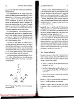
The first stages of query compilation are illustrated in Fig.
16.1.
The four boxes
in that figure correspond to the first
two stages of Fig.
15.2.
We have isolated a
"preprocessing" step, which
we shall discuss in Section
16.1.3,
between parsing
and conversion to the initial logical query plan.
Query
Parser
&\
Section
16.1

Section
16.3
Preferred logical
query
plan
Figure
16.1:
From a query to a logical query plan
In this section, we discuss parsing of SQL and give rudiments of a grammar
that can be used for that language. Section
16.2
is a digression from the line
of query-compilation steps,
where we consider extensively the various laws or
transformations that apply to expressions of relational algebra. In Section
16.3.
we resume the query-compilation story. First, we consider horv a parse tree
is turned into an expression of relational algebra, which becomes our initial
logical query plan. Then, rve consider
ways in which certain transformations
of Section
16.2
can be applied in order to improve the query plan. rather rhan
simply to change the plan into an equivalent plan of ambiguous merit.
16.1.1
'Syntax Analysis and Parse Trees
The job of the parser is to take test written in a language such as SQL and
convert it to a
pame tree,
which is a tree n-hose 11odcs correspond to either:

1.
Atoms,
which are lexical ele~nents such
as
keywords (e.g.,
SELECT).
names
of attributes or relations, constants, parentheses, operators such as
+
or
<,
and other schema elements. or
2.
Syntactic
categories,
which are names for families of query subparts that
all play a similar role in a query.
1i7e shall represent syntactic categories
by triangular brackets around a descriptive name. For example, <SFW>
will be used to represent any query in the common select-from-where form,
and <Condition> will represent any expression that is
a
condition; i.e.,
it can follow WHERE in SQL.
If a node is an atom, then it has no children. Howel-er, if the node is
a
syntactic category, then its children are described by one of the
rules
of the
grammar for the language.

We shall present these ideas by example. The
details of
horv one designs grammars for a language, and how one "parses," i.e.,
turns a program or query into the correct parse tree, is properly the subject of
a course on compiling.'
16.1.2
A
Grammar
for
a Simple Subset
of
SQL
1Ve shall illustrate the parsing process by giving some rules that could be used
for a query language that is a subset of SQL.
\Ve shall include some remarks
about
~vhat additional rules would be necessary to produce
a
complete grammar
for SQL.
Queries
The syntactic category <Query> is intended to represent all well-formed queries
of SQL. Some of its rules are:
Sote that \ve use the symbol
:
:=
conventionally to mean %an be expressed
as

The first of these rules says that a query

can
be a select-from-where form;
we shall see the rules that describe <SF\tT> next. The second rule says that
a
querv can be a pair of parentheses surrouilding another query. In a full SQL
grammar. we lvould also nerd rules that allowed a query to be a single relation
or an expression
invol~ing relations and operations of various types, such as
UNION
and
JOIN.
Select-From-Where
Forlns
lie give the syntactic category <SF\f'> one rule:
<SFW>
::=
SELECT
<SelList> FROM <FromList>
WHERE
<Condition>
'Those unfamiliar with the subject may wish to examine
A.
V.
Xho,
R.
Sethi, and
J.
D.
Ullman. Comptlers: Princtples, Technzpues,
and

Tools.
Addison-\Vesley, Reading
I'fA,
1986,
although the examples of Section
16.1.2
should be sufficient to place parsing in
the
context
of
the query processor.
Please purchase PDF Split-Merge on www.verypdf.com to remove this watermark.
790
CH-4PTER
16.
THE
QC'ERY
COJiPILER
This rule allorvs a limited form of SQL query. It does not provide for the various
optional clauses such
as
GROUP BY, HAVING, or ORDER BY, nor for options such
as
DISTINCT after SELECT. Remember that a real SQL grammar would hare a
much more complex structure for select-from-where queries.
Note our convention that keywords are capitalized. The syntactic categories
<SelList> and <fiomList> represent lists that can follow SELECT and FROM,
respecti\~ely. We shall describe limited forms of such lists shortly. The syntactic
category <Condition> represents
SQL

conditions (expressions that are either
true or false);
we
shall give some simplified rules for this category later.
Select-Lists
These two rules say that a select-list can be any comma-separated list of at-
tributes: either
a
single attribute or an attribute, a comma, and
any
list of one
or more attributes. Note that in a full SQL grammar
we
would also need provi-
sion for expressions and aggregation functions in the select-list and for aliasing
of attributes and expressions.
From-Lists
Here, a from-list is defined to be any comma-separated list of relations. For
simplification, we omit the possibility that elements of a from-list can be ex-
pressions,
e.g.,
R
JOIN
S,
or even
a
select-from-where expression. Likewise, a
full SQL grammar would have to
provide for aliasing of relations mentioned in
the from-list; here, we do not allow a relation to be followed by the

name of a
tuple
variable representing that relation.
Conditions
The rules we shall use are:
<Condition>
::=
<Condition>
AND
<Condition>
<Condition>
::=
<Tuple>
IN
<Query>
<Condition>
::=
<Attribute>
=
<Attribute>
<Condition>
::=
<Attribute> LIKE <Pattern>
Althougli
we
have listed more rules for conditions than for other categories.
these rules only scratch the surface of the forms of conditions.
i17e
hare oinit-
ted rules introducing operators

OR,
NOT, and EXISTS, comparisolis other than
equality and LIKE, constant operands. and a number of other structures that
are needed in
a
full SQL grammar. In addition, although there are several
forms that a tuple may take, we shall introduce only the one rule for syntactic
category <Tuple> that says a tuple can be a single attribute:
Base Syntactic
Categories
Syntactic categories <fittribute>, <Relation>, and <Pattern> are special,
in that they are not defined by grammatical rules, but
by rules about the
atoms for
which they can stand. For example, in a parse tree, the one child
of <Attribute> can be any string of characters that identifies an attribute in
whatever database schema the query is issued. Similarly, <Relation> can be
replaced by any string of characters that makes sense
as
a relation in the current
schema, and <Pattern> can be replaced by any quoted string that is
a
legal
SQL pattern.
Example
16.1
:
Our study of the parsing and query rewriting phase will center
around
twx-o versions of a query about relations of the running movies example:

StarsIn(movieTitle, movieyear, starName)
MovieStar(name, address, gender, birthdate)
Both variations of the query
ask
for the titles of movies that have at least one
star born in 1960.
n'e identify stars born in 1960 by asking if their birthdate
(an SQL string) ends in
'19602,
using the LIKE operator.
One way to ask this query is to construct the set of names of those stars
born in 1960 as a
subquery, and
ask
about each StarsIn tuple whether the
starName in that tuple is a member of the set returned by this subquery. The
SQL for this variation of the query is
sllo~vn in Fig. 16.2.
SELECT
movieTitle
FROM StarsIn
WHERE
starName
IN
(
SELECT name
FROM
Moviestar
WHERE birthdate LIKE
'%1960'

1;
Figure
16.2:
Find the movies with stars born in 1960
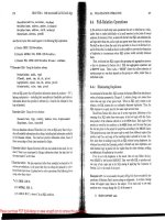
The parse tree for the query of Fig.
16.2,
according to the grammar n-e have
sketched, is shown in Fig.
16.3.
At the root is the syntactic category <Query>,
as must be the case for any parse tree of a query. Working down the tree,
we
see that this query is a select-from-ivhere form; the select-list consists of only
the attribute title, and the from-list is only the one relation
StarsIn.
Please purchase PDF Split-Merge on www.verypdf.com to remove this watermark.
792
CH-4PTER
16.
THE
QUERY COiWLER
16.1.
P.4
RSIAiG
793
SELECT movieTitle
FROM
StarsIn,
MovieStar
<SFW>

WHERE
starName
=
name
AND
//\\
birthdate
LIKE
'%19601;
SELECT <SelList>
FROM
<FromList> WHERE <Condition>
/
/
//
\
Figure 16.4: .&nother way to
ask
for the movies with stars born in 1960
<Attribute> <RelName> euple> IN <Query>
I
I
I
//\
movieTitle
<SFW>
starName <SW>
//\
SELECT <SelList> FROM <FromLisu WHERE <Condition>
/

/
//\
movieTitle StarsIn <RelName>
name Moviestar birthdate
'
%19601
Figure 16.3: The parse t,ree for Fig. 16.2
The condition in the outer WHERE-clause is more complex. It has the form
of tuple-IN-query, and the query itself is a parenthesized subquery, since all
subqueries must be surrounded by parentheses in
SQL.
The subquery itself is
another
select-from-where form, with its own singleton select- and from-lists
and a simple condition involving a
LIKE
operator.
Example
16.2:
Kow, let us consider another version of the query of Fig. 16.2.
this time without using a subquery.
We may instead equijoin thc relations
StarsIn
and
noviestar,
using the condition
starName
=
name,
to require that

the star mentioned in both relations be the same.
Note that
starName
is an
attribute of relation
StarsIn,
while
name
is an attribute of
MovieStar.
This
form of the query of Fig. 16.2
is
shown in Fig. 16.4.'
The parse tree for Fig. 16.1 is seen in Fig. 16.5. Many of the rules used
in
this parse tree are the same
as
in Fig. 16.3. However, notice how a from-list
with
Inore than one relation is expressed in the tree, and also observe holv a
condition can be several smaller conditions connected by an operator.
AND
in
this case.
n
<Attribute>
=
<Atmbute> <Attribute> LIKE <Pattern>
I

I
I I
starName name birthdate
'%1960f
Figure 16.5: The parse tree for Fig.
16.4
16.1.3
The
Preprocessor
What 11-e termed the
preprocessor
in Fig. 16.1 has several important functions.
If
a relation used in the query is actually a view, then each use of this relation
in the from-list must be replaced by a parse tree that describes the view. This
parse tree is obtained
from the definition of the viexv: which is essentially a
query.
The preprocessor is also responsible for
semantic checking.
El-en if the query
is valid syntactically, it actually may violate one or more semantic rules on the
use of names. For instance, the preprocessor must:
1.
Check relation uses.
Every relati011 mentioned in
a
FROM-clause must be
is
a

small difference between the t\vo queries in that
Fig.
16.4 can produce duplicates
if a
has
more than one star born in 1960. Strictly speaking, we should add
DISTINCT
a relation or view in the schema against which the query is executed.
to
Fig.
16.4,
but our example grammar
was
simplified to the extent of omitting that option.
For instance, the preprocessor applied to the parse tree of Fig. 16.3 dl
Please purchase PDF Split-Merge on www.verypdf.com to remove this watermark.
794
CHAPTER
16.
THE QUERY COMPILER
check that the t.wvo relations StarsIn and Moviestar, mentioned in the
two from-lists, are legitimate relations in the schema.
2.
Check and resolve attribute uses.
Every attribute that is mentioned in
the SELECT- or WHERE-clause
must be an attribute of some relation in
the current scope; if not, the parser must signal an error. For instance,
attribute title in the first select-list of Fig.
16.3 is in the scope of only

relation StarsIn. Fortunately, title is an attribute of
StarsIn, so the
preprocessor validates this use of title. The typical query processor
would at this point
resolve
each attribute by attaching to it the relation
to
which it refers, if that relation
was
not attached explicitly in the query
(e.g., StarsIn. title). It would also check ambiguity, signaling an error
if the attribute is in the scope of
two or more relations with that attribute.
3.
Check types.
A11 attributes must be of a type appropriate to their uses.
For instance, birthdate in Fig. 16.3 is used in a LIKE comparison,
wvhich
requires that birthdate be
a
string or
a
type that can be coerced to
a string. Since birthdate is a date, and dates in SQL can normally be
treated
as
strings, this use of an attribute is validated. Likewise, operators
are checked to see that they apply to values of appropriate and compatible
types.
If the parse tree passes all these tests, then it is said to be

valid,
and the
tree, modified by possible
view expansion, and with attribute uses resolved, is
given to the logical query-plan generator. If the parse tree is not valid, then an
appropriate diagnostic is issued, and no further processing occurs.
16.1.4
Exercises
for
Section
16.1
Exercise
16.1.1:
Add to or modify the rules for <SF\V> to include simple
versions of the following features of
SQL
select-from-where expressions:
*
a) The abdity to produce a set with the DISTINCT keyword.
b) -4 GROUP
BY
clause and a
HAVING
clause.
c) Sorted output
with the ORDER
BY
clause.
d)
.A

query with no \I-here-clause.
Exercise
16.1.2:
Add to tlie rules for <Condition> to allolv the folio\\-ing
features of SQL conditionals:
*
a)
Logical operators
OR
and
KOT
b)
Comparisons other than
=.
c) Parenthesized conditions.
16.2.
ALGEBRAIC
LAI4T.S
FOR
IAIPROVING QUERY
PLANS
795
d)
EXISTS
expressions.
Exercise
16.1.3:
Using the simple SQL grammar exhibited in this section,
give parse trees for the
following queries about relations

R(a,
b)
and
S(b,c):
a)
SELECTa,
c
FROM
R,
SWHERER.b=S.b;
b)
SELECT
a
FROM
R
WHERE
b
IN
(SELECT
a
FROM
R,
S WERE R.b
=
S.b);
16.2
Algebraic
Laws
for
Improving Query

Plans
We resume our discussion of the query compiler in Section
16.3,
where we first
transform the parse tree into an expression that is
wholly or mostly operators of
the extended relational algebra from Sections
5.2
and
5.4.
Also in Section
16.3,
we see hoxv to apply heuristics that we hope will improve the algebraic expres-
sion of the query, using some of the many algebraic
laws that hold for relational
algebra.
-4s a preliminary. this section catalogs algebraic laws that turn one ex-
pression tree into an equivalent expression tree that
maJr have a more efficient
physical query plan.
The result of applying these algebraic transformations is the logical query
plan
that is the output of the query-relvrite phase. The logical query plan is
then
conr-erted to a physical query plan.
as
the optinlizer makes a series of
decisions about implementation of operators. Physical query-plan
gelleration is
taken up starting

wit11 Section 16.4. An alternative (not much used in practice)
is for the
query-rexvrite phase to generate several good logical plans, and for
physical plans generated
fro111 each of these to be considered when choosing the
best overall physical plan.
16.2.1
Commutative and Associative Laws
The most common algebraic Iaxvs. used for simplifying expressions of all kinds.
are
commutati~e and associati\-e laws.
X
commutative
law
about an operator
says that it does not matter in
11-hicll order you present the arguments of the
operator: the result
will be the same. For instance,
+
and
x
are commutatix~
operators of arithmetic. More ~recisely,
x
+
y
=
y
+

x
and
x
x
y
=
y
X.X
for
any
numbers
1:
and
y.
On tlie other hand,
-
is not a commutative arithmetic
operator:
u
-
y
#
y
-
2.
.in
assoclatit:e
law
about an operator says that Fve may group t~o uses of the
operator either from

the left or the right. For instance.
+
and
x
are associative
arithmetic operators. meaning that
(.c
+
y)
+
z
=
.z
f
(9
+
2)
and
(x
x
y)
x
t
=
x
x
(y
x
z).
On

the other hand.
-
is not associative:
(x
-
y)
-
z
#
x
-
(y
-
i).
When an operator is both associative and commutative, then any number of
operands connected by this operator can be grouped and ordered as we wish
wit hour changing the result. For example,
((w
+
z)
+
Y)
+
t
=
(Y
+
x)
+
(Z

+
W)
.
Please purchase PDF Split-Merge on www.verypdf.com to remove this watermark.
CHAPTER
16.
THE QUERY COhfPILER
16.2.
ALGEBRAIC
LAWS
FOR IhIPROVLNG QUERY
PLAXS
797
Several of the operators of relational algebra are both associative and com-
mutative. Particularly:
Note that these laws hold for both sets and bags.
We shall not prove each of these laws, although we give one example of
a proof, below. The general method for verifying an algebraic
law involving
relations is to check that every tuple produced by the expression on the left
must also be produced by the expression on the right, and also that every tuple
produced on the right is likewise produced on the left.
Example
16.3:
Let us verify the commutative law for
w
:
R
w
S

=
S
w
R.
First, suppose a tuple
t
is in the result of
R
w
S, the expression on the left.
Then there must be
a
tuple
T
in
R
and a tuple
s
in
S
that agree with
t
on every
attribute that each shares with
t.
Thus, when we evaluate the espression on
the right,
S
w
R,

the tuples
s
and
r
will again combine to form
t.
We might imagine that the order of components of
t
will be different on the
left and right, but formally, tuples in relational algebra have no
fixed order of
attributes. Rather, we are free to reorder components, as long as
~ve carry the
proper attributes along in the column headers,
as
was discussed in Section
3.1.5.
We are not done yet with the proof. Since our relational algebra is an algebra
of bags, not sets, we must also verify that if
t
appears
n
times on the left then
it appears
n
times on the right, and vice-versa. Suppose
t
appears
n
times on

the left. Then it must be that the tuple
r
from
R
that agrees with
t
appears
some number of times
nR,
and the tuple
s
from
S
that agrees with
t
appears
some
ns
times, where
n~ns
=
n.
Then when we evaluate the expression
S
w
R
011
the right, we find that
s
appears

ns
times, and
T
appears
nR
times, so \re
get
nsnR
copies oft, or
n
copies.
We are still not done. We have finished the half of the proof that says
everything on the left appears on the right, but Ive must show that everything.
on the right appears on
tlie left. Because of the obvious symmetry, tlie argument
is essentially the same, and
we shall not go through the details here.
\Ve did not include the theta-join among the associative-commutatiw oper-
ators. True, this operator is commutative:
R~s=s~R.
Sloreover, if the conditions involved make sense where they are positioned, then
the theta-join is associative. However, there are examples, such as the
follo~t-ing.
n-here we cannot apply the associative law because the conditions do not apply
to attributes of the relations being joined.
I
Laws
for
Bags and Sets Can Differ
I

We should be careful about trying to apply familiar laws about sets to
relations that are bags. For instance, you may have learned set-theoretic
laws such
as
A
ns
(B
US
C)
=
(A
ns
B)
Us
(A
ns
C),
which is formally
the
"distributiye law of intersection over union." This law holds for sets,
but not for bags.
As an example, suppose bags
A,
B,
and
C
were each {x). Then
A
n~
(B

us
C)
=
{x)
ng
{x,x)
=
{x).
But
(A
ns
B)
UB
(A
n~
C)
=
{x)
Ub
{x)
=
{x, x), which differs from the left-hand-side, {x).
Example
16.4
:
Suppose we have three relations
R(a,
b),
S(b,c),
and

T(c,
d).
The expression
is transformed by a hypothetical associative
law into:
However, \ve cannot join
S
and
T
using tlie condition
a
<
d,
because
a
is an
attribute of neither
S
nor
T.
Thus, the associative law for theta-join cannot be
applied arbitrarily.
16.2.2
Laws Involving Selection
Selections are crucial operations from the point of view of query optimization.
Since selections tend to reduce the size of relations markedly, one of the most
important rules of efficient query processing is to move the selections down the
tree as far as they
~i-ill go without changing what the expression does. Indeed
early query optimizers used variants of this transformation

as
their primary
strategy for selecting good logical query plans.
.As we shall point out shortly, the
transformation of
.'push selections down the tree" is not quite general enough,
1
but the idea of .'pushing selections" is still a major tool for the query optimizer.
I
In this section 11-e shall studv the law involving the
o
operator. To start,
~vhen the condition of a selection is complex (i.e., it involves conditions con-
nccted by
AND
or
OR).
it helps to break the condition into its constituent parts.
The
motiration is that one part, involving felver attributes than the whole con-
dition.
ma)- be ma-ed to a convenient place that the entire condition cannot
go. Thus; our first
tiyo laws for
cr
are the
splitting
laws:
oC1
AND

C2
(R)
=
UCl
(ffc2
(R)).
Please purchase PDF Split-Merge on www.verypdf.com to remove this watermark.
798
CHAPTER
16.
THE
QUERY CO,%fPILER
However, the second law, for
OR,
works only if the relation
R
is a set. KO-
tice that if
R
were a bag, the set-union would hase the effect of eliminating
duplicates incorrectly.
Notice that the order of
C1 and Cz is flexible. For example, we could just as
u-ell have written the first law above with C2 applied after CI,
as
a=, (uc, (R)).
In fact, more generally, we can swap the order of any sequence of
a
operators:
gel

(oc2 (R))
=
5c2
(ac,
(R))
.
Example
16.5
:
Let
R(a,
b,
c)
be a relation. Then
OR
a=3)
AND
b<c
(R)
can
be split
as
aa=l
OR
.=3(17b<~(R)).
We can then split this expression at the
OR
into
(Ta=l (u~<~(R))
U

~a=3(ob<c(R)).
In this case, because it is impossible for
a
tuple to satisfy both
a
=
1
and
a
=
3,
this transformation holds regardless
of
whether or not
R
is a set,
as
long
as
Ug
is used for the union. However, in
general the splitting of
an
OR
requires that the argument be a set and that
Us
be used.
Alternatively, we could have started to split by making
ob,,
the outer op-

eration, as
UF,<~
(5.~1
OR
a=3(R)).
When me then split the OR, we \vould get
U~<C(U~=~(R)
U
oa=3(R)),
an
expression that is equivalent to, but somewhat
different from the first expression we derived.
The next family of laws involving
o
allow us to push selections through the
binary operators: product, union, intersection, difference, and join. There are
three types of laws, depending on whether it is optional or required to push the
selection to each of the arguments:
1.
For a union, the selection
must
be pushed to both arguments.
2.
For
a
difference, the selection must be pushed to the first argument and
optionally may be pushed to the second.
3.
For the other operators it is only required that the selection be pushed
to one argument. For joins and products, it may not make sense to push

the selection to both arguments, since an argument may or may not have
the attributes that the selection requires.
When it is possible to push to
both, it
may or may not improve the plan to do so; see Exercise
16.2.1.
Thus, the law for union is:
Here, it is mandatory to
move the selection down both branches of the tree.
For difference, one version of the law is:
Ho~vever, it is also permissible to push the selection to both arguments, as:
16.2.
ALGEBR4IC
LAWS
FOR 1hIPROVING QUERY
PLANS
The next laws allow the selection to be pushed to one or both arguments.
If the selection is
UC,
then we can only push this selection to a relation that
has all the attributes mentioned in
C, if there is one. \\'e shall show the laws
below assuming that the relation
R
has all the attributes mentioned in
C.
oc (R
w
S)
=

uc
(R)
w
S.
If C
has
only attributes of
S,
then we can instead write:
and similarly for the other three operators
w,
[;;1,
and
n.
Should relations
R
and
S
both happen to have all attributes of
C,
then we can use laws such
as:
Note that it is impossible for this variant to apply if the operator
is
x
or
z,
since in those cases
R
and

S
have no shared attributes. On the other halld, for
n
the law always applies since the sche~nas of
R
and
S
must then be the same.
Example
16.6
:
Consider relations
R(a,
b)
and
S(b,
c) and the expression
The condition
b
<
c
can be applied to
S
alone, and the condition
a
=
1
OR
a
=

3
can be applied to
R
alone. We thus begin by splitting the
AND
of the two
conditions as we did in the first alternative of Example
16.5:
Xest, we can push the selection
a<,
to
S,
giving us the expression:
Lastly,
we push the first condition to
R.
yielding:
U.=I
OR
.=3(R)
w
ub<=(S).
Optionally, \r.e can split the
OR
of txvo conditions
as
ne did in Example
16.5.
However, it may or may not be advantageous to do so.
Please purchase PDF Split-Merge on www.verypdf.com to remove this watermark.

800
CHAPTER
16.
THE
QUERY
COAIPILER
Some Trivial
Laws
We are not going to state every true law for the relational algebra. The
reader should be alert, in particular, for laws about extreme cases: a
relation that is empty, a selection or theta-join whose condition is
always
true or always false, or a projection onto the list of all attributes, for
example.
A
few of the many possible special-case laws:
Any selection on an empty relation is empty.
If
C
is an always-true condition (e.g.,
x
>
10
OR
x
5
10
on a relation
that forbids
x

=
NULL),
then uc(R)
=
R.
If
R
is empty, then
R
U
S
=
S.
L
16.2.3
Pushing
Selections
As
was
illustrated in Example
6.52,
pushing a selection down an expression
tree
-
that is, replacing the left side of one of the rules in Section
16.2.2
by
its right side
-
is one of the most powerful tools of the query optimizer. It

was long assumed that we could optimize by applying the laws for
u only in
that direction.
Horvcver, when systems that supported the use of viem became
common, it was found that in some situations it was essential first to move a
selection as far
up
the tree
as
it would go, and then push the selections down all
possible branches.
-4n example should illustrate the proper selection-pushing
approach.
Example
16.7:
Suppose we have the relations
StarsIn(title, year, starName)
Movie(title, year, length, incolor, studioName, producerC#)
Sote that we have altered the first two attributes of
StarsIn
from the usual
movieTitle
and
movieyear
to make this example simpler to follow. Define
view
MoviesDf 1996
by:
CREATE VIEW MoviesOfl996 AS
SELECT

*
FROM Movie
,WHERE year
=
1996;
We
can
ask
the query "which stars worked for which studios in
199G?"
by the
SQL query:
16.2.
ALGEBRAIC
LA1V.S
FOR
IhiPROVIArG
QUERY
PLALVS
SELECT starName, studioName
FROM MoviesOfl996 NATURAL JOIN StarsIn;
The view
MoviesOf 1996
is defined
by
the relational-algebra expression
Thus, the query. which is the natural join of this expression with
StarsIn,
follo~ved by a projection onto attributes
starName

and
studioName,
has the
expression, or '.logical query plan," shown in Fig.
16.6.
OYeur=
1996
StarsIn
I
Movie
Figure 16.6: Logical query plan constructed from definition of a query and view
In this expression. the one selection is already as far down the tree as it will
go,
so
there is
IIO
11-a\- to .Lpush selections don-n the tree." However, the rule
uc(R
w
S)
=
gc(R)
w
S
can
bc
applied ,.back~~-ards." to bring the selection
uy,,,=l99o
above the join in Fig.
1G.6.

Then. since
year
is an attribute of both
Movie
and
StarsIn.
we may push the selection doix-n to
both
children of the
join node. The resulting logical
query plan is shown in Fig.
16.7.
It is likely to
be
an impro~ement. since we reduce the size of the relation
StarsIn
before rve
join it with the molies
of
1996.
Movie
StarsIn
Figure
16.7:
Ilnprorillg the query plan
by
moving selections up and down the
tree
Please purchase PDF Split-Merge on www.verypdf.com to remove this watermark.
802

CHAPTER
16.
THE
QUERY COhIPZLER
16.2.4
Laws
Involving Projection
Projections, like selections, can be "pushed down" through many other opera-
tors. Pushing projections differs from pushing selections in that when we push
projections, it is quite usual for the projection also to remain where it is. Put
another way, "pushing" projections really involves introducing a new projection
somewhere below an existing projection.
Pushing projections is useful, but generally less so than pushing selections.
The reason is that while selections often reduce the size of a relation by a large
factor, projection keeps the number of tuples the same and only reduces the
length of tuples. In fact, the extended projection operator of Section
5.4.5
can
actually increase the length of tuples.
To describe the transformations of extended projection, we need to introduce
some terminology. Consider a term
E
+
x
on the list for a projection, where
E
is an attribute or an expression involving attributes and constants. We say
all attributes mentioned in
E
are

input
attributes of the projection, and
x
is an
output
attribute. If a term is
a
single attribute, then it is both an input and
output attrihute. Note that it is not possible to have an expression other than
a single attribute without an arrow and renaming, so
we have covered all the
cases.
If a projection list consists only of attributes, with no renaming or expres-
sions other than a single attribute, then
11-e
say the projection is simple. In the
classical relational algebra, all projections are simple.
Example
16.8
:
Projection
T~,~,~(R)
is simple;
a,
b,
and
c
are both its input
attributes and its output attributes. On the other hand,
ra+b+=, JR)

is not
simple. It has input attributes a,
b,
and
c.
and its output attributes are
x
and
c.
The principle behind laws for projection is that:
We may introduce a projection anywhere in an expression tree, as long as
it eliminates only attributes that are never used by any of the operators
above, and are not in the result of the entire expression.
In the most basic form of these laws, the introduced projections are
alw-ays
simple, although other projections, such as
L
below, need not be.
xL(R
w
S)
=
n~ (nnj(R)
w
n,v(S)).
~vhere
dl
is the list of all attributes
of
R

that are either join attributes (in the schema of both
R
ant1
S)
or are
input attributes of
L,
and
iY
is the list of attributes of
S
that are cither
join attributes or input attributes of
L.
~L(R
S)
=
~L(wnf(R)
7
.ii~(S)).
\,-here
A1
is the list of all attributes
of
R
that are either join attributes (i.e., are mentioned in condition
C)
or are input attributes of
L,
and

N
is the list of attributes of
S
that are
either join attributes or input attributes of
L.
16.2.
ALGEBRAIC
LAlVS
FOR I3.iPROVliVG
QUERY
PLANS
803
xt(R
x
S)
=
nt(nAf(R)
x
nN(S)),
where
hf
and
N
are the lists of all
attributes of
R
and
S,
respectively, that are input attributes of

L.
Example
16.9:
Let
R(a,
b,
c)
and
S(c,
d,
e)
be two relations. Consider the
expression
x,+,,,, b+y(R
w
S).
The input attributes of the projection are a,
b,
and e, and
c
is the only join attribute. We may apply the law for pushing
projections
belorv joins to get the equivalent expression:
Sotice that the projection
Z,,~,~(R)
is trivial; it projects onto all the at-
tributes of
R.
We may thus eliminate this projection and get a third equivalent
expression:

T=+~.+~,
b-+y (R
w
rC,,(S)).
That is, the only change from the
original is that we remove the attribute
d
from
S
before the join.
In addition, we can perform a projection entirely before a bag union. That
is:
On the other hand, projections cannot be pushed below set unions or either the
set or bag versions of intersection or difference at all.
Example
16.10
:
Let
R(a,
b) consist of the one tuple
((1,211
and
S(a,
b)
consist of the one tuple
((1.3)).
Then
na(R
fl
S)

=
~~(0)
=
0.
However,
a
a
=
1
1
=
1)
If the projection involves some computations, and the input attributes of
a term
on the projection list belong entirely to one of the arguments of a join
or product
bclo~r- the projection; then we have the option, although not the
obligation, to perform the computation directly on that argument.
An example
should help illustrate the point.
Example
16.11
:
Again let
R(a,
b.
c)
and
S(c,
d,

e)
be relations, and consider
the join and projection
iio+b+x,
d+c-+y(R
w
S).
IVe can more the sum
a
+
b
and its renaming to
.t.
directly onto the relation
R,
and move the sum
d
+
e
to
S
similarly. The resulti~lg equivalent expression is
One special case to handle is if
r
or
y
\r-ere
c.
Then. we could not rename
a sun1 to

c.
because a relation cannot have two attributes named c.
Thus.
we ~ould have to invent a temporary name and do another renaming in the
projection above the join. For example,
ii,+~,+~,
d+e ty(R
w
S)
could become
ii:+c.
y(~a+b-+:,
c(R)
rd+e+y. c(S)).
It is also possible to push a projection below a selection.
Please purchase PDF Split-Merge on www.verypdf.com to remove this watermark.
804
CHAPTER
16.
THE
QUERY COiWILER
m(nc(R))
=
rr,
(U~(~M(R))), where
M
is the list of all attributes that
are either input attributes of
L
or mentioned in condition

C.
As in Example 16.11, we have the option of performing computations on the
list
L
in the list
111
instead, provided the condition
C
does not need the input
attributes of
L
that are involved in a computation.
Often, we wish to push projections down expression trees, even if
we have to
leave another projection above, because projections tend to reduce the size of
tuples and therefore to reduce the number of blocks occupied by an intermediate
relation. However:
we must be careful when doing so, because there are some
common examples where pushing a projection down costs time.
Example
16.12:
Consider the query asking for those stars that worked in
1996:
SELECT starName
FROM
StarsIn
WHERE
year
=
1996;

about the relation
StarsIn(movieTitle, movieyear, starName).
The direct
translation of this query to a logical query plan is shown in Fig. 16.8.
starName
I
movieyear=
1996
I
StarsIn
Figure 16.8: Logical query plan for the query of Example 16.12
We can add below the selection a projection onto the attributes
1.
starName,
because that attribute is needed in the result, and
2.
movieyear,
because that attribute is needed for the selection condition.
The result is
shown in Fig. 16.9.
If
StarsIn
were not a stored relation. but a relation that was constructed
by another opmation.
sucll as
a
join, then the plan of Fig. 16.9 makes sense.
Ue can "pipeline" the projection (see Section
16.7.3)
as tuples of the join are

generated, by simply dropping
the useless
title
attribute.
However: in this case
StarsIn
is a stored relation. The lower projection in
Fig. 16.9 could actually waste a lot of time, especially if there were an index
on
movieyear.
Then a physical query plan based on the logical query plan of
Fig. 16.8 would first
use
the index to get only those tuples of
StarsIn
that have
movieyear
equal to 1996, presumably a small fraction of the tuples. If we do
16.2.
ALGEBRAIC
LAI,\fS
FOR IMPROVII\~G
QUERY
PLAlVS
I
'
srarNarne, movieYear
I
StarsIn
Figure 16.9: Result of introducing a projection

the projection first,
as
in Fig. 16.9, then we have to read every tuple of
StarsIn
and project it. To make matters worse, the index on
movieyear
is probably
useless in the projected
relati011
~,~~,,~,,,,,~,,~~~(~tarsIn),
SO
the selection
now involves a scan of all the tuples that result from the projection.
16.2.5
Laws About
Joins
and Products
lie
saw in Section 16.2.1 many of the important laws involving joins and prod-
ucts: their
commutative and associative laws. However, there are a few addi-
tional
laws that follow directly from the definition of the join, as was mentioned
in Section
5.2.10.
R
w
S
=
z~(u~(R

x
S)),
where
C
is the condition that equates each
pair of attributes from
R
and
S
with the same name. and
L
is a list that
includes one attribute from each equated pair and all the other attributes
of
R
and
S.
In practice. we usually want to apply these rules from right to left. That is, ae
identify a product followed by a selection as a join of some kind. The reason for
doing so is
that the algorithnls for computillg joins are generally much faster
than algorithms that
colnplite a product follo~vcd by a selection on the (rery
large) result
of
the product.
16.2.6 Laws Involving Duplicate Elimination
The operator
6.
\vhich elinli~lates duplicates from a bag. can be pushed through

many. but not all operators. In general, moving a
6
down the tree reduces the
size of
intermediate relations and may therefore be beneficial. Sloreover, we
can sometimes niol-e the
d
to a position where it can be eliminated altogether,
because it is applied to a relation that is
known not to possess duplicates:
6(R)
=
R if R has no duplicates. Important cases of such a relation
R
include
Please purchase PDF Split-Merge on www.verypdf.com to remove this watermark.
806
CH-4PTER
16.
THE
QUERY C0:ViPILER
a)
A
stored relation with a declared primary key, and
b)
A
relation that is the result of
a
7
operation, since grouping creates

a
relation with no duplicates.
Several laws that "push" 6 through other operators are:
We can also move the
6
to either or both of the arguments of an intersection:
On
the other hand,
6
cannot be moved across the operators
UB,
-8,
or
7i
in
general.
Example
16.13
:
Let R have two copies of the tuple
t
and
S
have one copy of
t.
Then 6(R
Ug
S) has one copy of
t,
while 6(R)

UB
B(S) has two copies of
t.
Also, 6(R
-B
S) has one copy oft, while 6(R)
-B
6(S) has no copy oft.
Xow, consider relation
T(a.
b)
with one copy each of the tuples (1,2) and
(1,3), and no other tuples. Then 6(xir,(T)) has one copy of the tuple (I), while
w,
(S(T)) has tn-o copies of (1).
Finally, note that commuting
6
with
Us.
fls,
or
-s
makes no sense. Since
producing a set is one
way to guarantee there are no duplicates, Ive can eliminate
the
6
instead. For example:
-
Sote, however, that a11 implementation of

Us
or the other set operators in-
volves
a
duplicate-elimination process that is tantamount to applying 6; see
Section 15.2.3, for example.
16.2.7
Laws Involving
Grouping
and Aggregation
IVllen we consiticr the operator
y,
we find that the applicability of many trans-
formations
depends on the details of the aggregate operators used. Thus. n-e
cannot statc laws in the generality that Ive used for the other operators. One
exception is the law, mentioned in Section
16.2.6, that
a
y
absorbs a
6.
Pre-
cisely:
16.2.
ALGEBRAIC
LA\,\:S
FOR
IAIPROVISG QL'ERY
PLANS

807
Another general rule is that
we
may project useless attributes from the ar-
gument should
~ve wish, prior to applying the
y
operation. This law can he
witten:
Yt(R)
=
y~(n~,~(R)) if
A6
is a list containing at least all those attributes
of
R
that are mentioned in L.
The reason that other transformations depend on the
aggregation(s) in-
rol\.ed in a
y
is that some aggregations
-
MIN
and
MAX
in particular
-
are not
affected by the presence or absence of duplicates. The other aggregations

-
SUM, COUNT, and
AVG
-
generally produce different values if duplicates are elim-
inated prior to application of the aggregation.
Thus, let us call an operator
y~
duplicate-impervious
if the only aggregations
in
L
are
MIN
and/or MAX. Then:
yL(R)
=
yL
(G(R)) provided
y~
is duplicate-impervious.
Example
16.14
:
Suppose we have the relations
MovieStar(name
,
addr
,
gender, birthdate)

StarsIn(movieTitle, movieyear, star~ame)
and we want to know for each year the birthdate of the youngest star to appear
in a
morie that year. lye can express this query as
SELECT
movieyear,
movi birth date)
FROM MovieStar, StarsIn
WHERE name
=
starName
GROUP
BY
movieyear;
Y
aoricYear,
MAX
(
birthdate
)
I
plante
=
starh'orne
I
/"\
MovieStar
StarsIn
Figure 16.10: Initial logical query plan for the query of Esa~nple 16.11
.in initial logical quely plan constructed directly from the query is sho~rn

in Fig. 16.10. The FROM list is expressed by a product, and the WHERE clause
by
a selection abore it. The grouping and aggregation are expressed by the
y
operator above those. Some transformations that we could apply to Fig. 16.10
if
we nished are:
Please purchase PDF Split-Merge on www.verypdf.com to remove this watermark.
808
CHAPTER
16.
THE
QUERY
COkIPILER
1.
Combine the selection and product into an equijoin.
2.
Generate
a
6 below the
y,
since the
y
is duplicate-impervious.
3.
Generate
a
T
between the
and the introduced

6
to project onto
movie-
Year
and
birthdate,
the only attributes relevant to the
?.
The resulting plan is shown in Fig.
16.11.
MovieStar StarsIn
Figure
16.11:
Another query plan for the query of Example
16.14
We can now push the
6
belo\\, the
w
and introduce v's below that if n-e n-ish.
This new query plan is shown in Fig.
16.12.
If
name
is a key for
MovieStar.
the
6
can be eliminated along the branch leading to that relation.
MovieStar

StarsIn
Figure
16.12:
X
third query plan for Example
16.11
16.2.
rlLGEBR=LIC
LA115
FOR
IhfPROlrIArG QUERY
PLdSS
809
16.2.8
Exercises
for
Section
16.2
*
Exercise
16.2.1
:
When it is possible to push
a
selection to both arguments
of a binary operator, we need to decide whether or not to do so. How would
the existence of indexes on one of the arguments affect our choice? Consider,
for instance, an expression
oc(R
n

S),
where there is an index on
S.
Exercise
16.2.2
:
Give examples to show that:
*
a) Projection cannot be pushed below set union.
b)
Projection cannot be pushed below set or bag difference.
c) Duplicate elimination (6) cannot be pushed below projection.
d) Duplicate elimination cannot be pushed below bag union or difference.
!
Exercise
16.2.3
:
Prove that we can always push
a
projection below both
branches of a bag union.
!
Exercise
16.2.4:
Some la~x-s that hold for sets hold for bags; others do not.
For each of the
laws below that are true for sets; tell whether or not it is true
for bags. Either give a proof the law for bags is true, or
give
a

counterexample.
*
a)
R
U
R
=
R
(the idempotent law for union).
b)
R
rl
R
=
R
(the idempotent law for intersection).
d)
R
u
(S
n
T)
=
(R
IJ
S)
17
(R
u
T)

(distribution of union over intersec-
tion).
!
Exercise
16.2.5:
lye can define
for bags by:
R
S
if and only
if
for every
element
x.
the number of times
x
appears in
R
is less than or equal to the
number of times it appears in
S.
Tell rvhether the follolr-ing statements (which
are all true for sets) are
true for bags: give either a proof or
a
counterexample:
a) If
RE
S:
then

RUS=
S.
c)
If
RE
Sand
S
g
R.
then
R=
S.
Exercise
16.2.6
:
Starting with an expressio~l
i~r.
(R(a.
b.
c)
w
S(b:
c:
d,
e)),
push the projection down as far as it can go if
L
is:
Please purchase PDF Split-Merge on www.verypdf.com to remove this watermark.
810

CHAPTER
16.
THE
QUERY COAlPILER
!
Exercise
16.2.7:
We mentioned in Example 16.14 that none of the plans
w
showed is necessarily the best plan. Can you think of a better plan?
!
Exercise
16.2.8
:
The following are possible equalities involving operations on
a relation
R(a,
b).
Tell whether or not they are true; give either a proof or a
counterexample.
!!
Exercise
16.2.9:
The join-like operators of Exercise
15.2.4
obey some of the
familiar laws, and others do not. Tell whether each of the following is or is not
true.
Give
either a proof that the law holds or a counterexample.

C)
uc(R
&I,
S)
=
uc(R)
AL
S, where
C
involves only attributes of
R.
d)
uc(R
At
S)
=
R
DFjL
uC(S),
where
C
involves only attributes of
3.
*f)
(R&
S)
AT
=R
cfb
(S

DFj
T).
16.3
From
Parse
Trees
to
Logical
Query
Plans
Ke now resume our discussion of the query compiler. Having constructed a
parse tree for a query in Section 16.1,
we nest need to turn the Darse tree
into the preferred logical query plan. There are
two steps, as was suggested in
Fig. 16.1.
The first step is to replace the nodes and structures of the parse tree. in
appropriate groups, by an operator or operators of relational algebra.
\Ye
shall
suggest some of these rules
and
leave some others for exercises. The second step
is to take the relational-algebra expression produced by
tlie first step and to
turn it into an expression that
we expect can be converted to the most efficient
physical query plan.
16.3.
FROM

PARSE
TREES
TO LOGICAL
QUERY
PLrlNS
811
16.3.1
Conversion
to
Relational Algebra
We shall now describe informally some rules for
transforming
SQL
parse trees to
algebraic logical query plans. The first rule, perhaps the most important, allows
us to convert all "simple" select-from-where constructs to relational algebra
directly. Its informal statement:
If I\-e have a <Query> that is a
<SF&'>
construct, and the <Condition>
in this construct has no subqueries, then we may replace the entire con-
struct
-
the select-list, from-list, and condition
-
by
a
relational-algebra
expression consisting, from bottom to top,
of:

1.
The product of all the
elations
mentioned in the <FromList>, which
is the argument
of:
2.
A
selection
ac,
where
C
is the <Condition> expression in the con-
struct being replaced, which in turn is the argument of:
3.
A
projection
n-L,
where
L
is the list of attributes in the <SelList>.
Example
16.15:
Let us consider the parse tree of Fig. 16.5. The select-
from-where transformation applies to the entire tree of Fig. 16.5. We take the
product of the
two relations
StarsIn
and
MovieStar

of the from-list, select for
the condition in the
subtree rooted at <Condition>: and project onto the select-
list,
movieTitle.
The resulting relational-algebra espression is Fig. 16.13.
IT
rrrovieTirle
I
(r
s,or~allle
=
rlarne
AVD
birthdore
LIKE
'
$1960
'
I
/"\
StarsIn
Moviestar
I
Figure 16.13: Translation of a parse tree to an algebraic expression tree
The same transformation does not apply to the outer query of Fig. 16.3.
The reason is that the condition involves a
subquery. \Ye shall discuss in Sec-
tion 16.3.2 how to deal
with conditions that have subqueries, and you should

esanline the bos on '.Lin~itations on Sclection Conditions" for an esplanation
of ~vhy 11-e make tlie distinction betwen conditions that ha~e subqueries and
those that do not.
Hen-ever,
ae could apply the select-from-\vhere rule to the subquery in
Fig. 16.3. The expression of relational algebra that
Re get from the subquery
is
~narne
(ubrrthdate
LIKE
'Xi960'
(~ovie~tar)).
Please purchase PDF Split-Merge on www.verypdf.com to remove this watermark.
812
CHAPTER
16.
THE
QUERY
COdfPILER
Limitations on Selection Conditions
One might wonder why we do not allow
C,
in a selection operator uc, to
involve a subquery. It is conventional in relational algebra for the
argu-
ments
of
an
operator

-
the elements that do not appear in subscripts
-
to be expressions that yield relations.
On
the other hand,
parameters
-
the elements that appear in subscripts
-
have a type othcr than rela-
tions. For instance, parameter
C
in
uc
is a boolean-valued condition, and
parameter
L
in
nL
is a list of attributes or formulas.
If we follow this convention, then whatever calculation is implied
by a
parameter can be applied to each tuple of the relation
argument(s). That
limitation on the use of parameters simplifies query optimization. Suppose,
in contrast, that we allowed an operator like
uc(R), where C involves a
subquery. Then the application of
C

to each tuple of
R
involves computing
the subquery. Do we compute it anew for every tuple of
R?
That ~ould,
be unnecessarily expensive, unless the subquery were
correlated,
i.e., its
value depends on something defined outside the query, as the
subquery of
Fig.
16.3
depends on the value of
starName.
Even correlated subqueries
can be evaluated without recomputation for each tuple, in most cases,
provided we organize the computation correctly.
16.3.2
Removing Subqueries From Conditions
For parse trees with a <Condition> that has a subquery, we shall introduce
an intermediate form of operator, between the syntactic categories of
the parse
tree and the relational-algebra operators that apply to relations. This operator
is often called
two-argument selection.
We shall represent a two-argument selec-
tion in a transformed parse tree by a node labeled a, with no parameter.
Beloiv
this node is a left child that represents the relation

R
upon ~vhicli the selection
is being performed, and a right child that is an expression for the
condition
applied to each tuple of
R.
Both arguments may be represented as parse trees.
as
expression trees, or
as
a mixture of the two.
Example
16.16:
In Fig.
16.14
is a rewriting of thc parse tree of Fig.
16.3
that uses a two-argument selection. Several transformations have been made
to construct Fig.
16.14
from Fig.
16.3:
1.
The
subquery in Fig.
16.3
has been replaccd hy an expression of relational
algebra, as discussed at the end of Example
16.15.
2.

The outer query has also been replaced. using the rule for select-from-
where expressions from Section
16.3.1.
However. we have expressed the
necessary selection
as
a tn-o-argument selection, rather than by the con-
ventional
a
operator of relational algebra. As a result, the upper node of
16.3.
FROM
P.4RSE
TREES
TO LOGICAL QUERY PLANS
StarsIn
<Condition>
4ttribute>
'
binkfote
LIKE
'
9.1960'
I
I
st
arName
Moviestar
Figure
16.14:

An expression using a two-argument
a,
midway between a parse
tree and relational algebra
the parse tree labeled <Condition> has not been replaced, but remains
as an argument of the selection, with part of
it.$
expression replaced by
relational algebra, per point
(1).
This tree needs further transformation, which we discuss next.
0
We need rules that allow us to replace a two-argument selection by
a
one-
argument selection and other operators of relational algebra. Each form of
condition
may require its own rule. In common situations, it is possible to re-
move the
two-argument selection and reach an expression that is pure relational
algebra. However, in extreme cases, the two-argument
selectio~l can be left in
place and considered part of the logical query plan.
We shall give. as an example, the rule that lets us deal with the condition in
Fig.
16.14
involving the
IN
operator. Note that the subquery in this condition is
uncorrelated: that is, the

subquery's relation can be computed once and for all,
independent of the tuple being tested. The rule for eliminating such a condition
is stated informally as
follorvs:
Suppose we have a two-argument selection in which the first argument
represents some relation
R
and the second argument is a <Condition> of
the form
t
IN
S. n-here expression
S
is an uncorrelated subquery: and
t
is a tuple co~nposed of (son~c) attributes of
R.
We transform the tree as
follo~i-s:
a) Replace the <Condition> by the tree that is the expression for
S.
If
S
may have duplicates, then it is necessary to include a
6
operation
at the root of the expression for S, so the expression being formed
does
not produce more copies of tuples than the original query does.
Please purchase PDF Split-Merge on www.verypdf.com to remove this watermark.

814
CHAPTER
16.
THE
QUERY
COMPILER
b) Replace the two-argument selection by a one-argument selection
oc,
where
C
is the condition that equates each component of the tuple
t
to the corresponding attribute of the relation
S.
c)
Give
oc
an argument that is the product of
R
and
S.
Figure 16.15 illustrates this transformation.
Figure
16.15: This rule handles a two-argument selection with
a
condition in-
volving
IN
Example
16.17:

Consider the tree of Fig. 16.14, to which we shall apply the
rule for
IN
conditions described above. In this figure, relation
R
is StarsIn,
and relation
S
is the result of the relational-algebra expression consisting of
the
subtree rooted at
T,,,,.
The tuple
t
has one component, the attribute
st
arName.
The two-argument selection is replaced by
(TstarName=name;
its condition
C
equates the one component of tuple
t
to the attribute of the result of query
S.
The child of the
a
node is a
x
node, and the arguments of the

x
node
are the node labeled StarsIn and the root of the expression for
S.
Sotice
that, because name is the key for MovieStar, there is no need to introduce a
duplicate-eliminating
d
in the expression for
S.
The new expression is shown
in Fig. 16.16. It is completely in relational algebra, and is equivalent to the
expression of Fig. 16.13, although its structure is quite different.
The strategy for translating subqueries to relational algebra is more com-
plex
when the subquery
is
correlated. Since correlated subqueries involve un-
known values defined outside themselves, they cannot be translated in isolation.
Rather,
we need to translate the subquery so that it produces a relation in n-hich
certain extra attributes appear
-
the attributes that must later be compared
~vith the esternally defined attributes. The conditions that relate attributes
from the
subquery to attributes outside are then applied to this relation. and
the extra attributes that are no longer necessary can then be projected out.
During this process,
we must be careful about accidentally introducing dupli-

cate tuples, if the query does not eliminate duplicates at the end. The following
example illustrates this technique.
16.3.
FROM
PARSE
TREES
TO
LOGICAL QUERY
PL-AXS
IL
movicTitle
I
W
sarName
=
name
StarsIn
nome
I
'
binhdare
LIKE
'
t1960'
I
MovieStar
Figure 16.16: Applying the rule for
IN
conditions
SELECT DISTINCT

ml.movieTitle, ml.movieYear
FROM
StarsIn
ml
WHERE ml.movieYear
-
40
<=
(
SELECT
AVG
(birthdate)
FROM StarsIn m2,
MovieStar s
WHERE m2.starName
=
s.name
AND
m1,movieTitle
=
m2,movieTitle
AND
ml.movieYear
=
m2.movieYear
);
Figure 16.17: Finding movies with high average star age
Example
16.18:
Figure 16.17 is an

SQL
rendition of the query: "find the
movies
where the average age of the stars
was
at most
40
when the movie was
made.'' To simplify, we treat birthdate as a birth year, so we can take its
average and get a
value that can be compared with the movieyear attribute of
StarsIn.
We have also written the query so that each of the three references
to relations has its own tuple variable. in order to help remind us where the
various attributes come from.
Fig. 16.18
sho\vs the result of parsing the query and performing a partial
translation to relational algebra. During this
initla1 translation, we split the
WHERE-clause of the
subquery in txvo. and used part of it to convert the product
of relations to an equijoin.
\Ye have retained the aliases ml, m2, and
s
in
the nodes of this tree, in order to make clearer the origin of each attribute.
Alternatively. we could have used projections to rename attributes and thus
avoid conflicting attribute names. but the result would be harder to
follo\v.
111 order to remove the <Condition> node and eliminate the two-argument

a,
we need to create an expression that describes the relation in the right
branch of the <Condition>.
Holvever. because the subquery is correlated, there
Please purchase PDF Split-Merge on www.verypdf.com to remove this watermark.
816
CHAPTER
16.
THE QUERY COMPILER
StarsIn ml
<Condition>
m1
'
40
'
m2.movieTitle
=
mI.mot~ieTitlc
AND
m2.movieYear
=
ml.nlovieYeor
I
Da
7~
StarsIn
m2
Moviestar
s
Figure 16.18: Partially transformed parse tree for Fig. 16.17

is no way to obtain the attributes
ml.movieTitle
or
ml .movieyear
froill the
relations mentioned in the subquery, which are
StarsIn
(with alias
m2)
and
MovieStar.
Thus,
we need to defer the selection
until after the relation from the
subquery is combined with the copy of
StarsIn
from the outer query (the copy aliased
nl).
To transform the logical quer>- plan
in this
way, we need to modify the
y
to group by the attributes
m2. movieTitle
and
m2.movie'iear,
so these attributes will be available when needed by the
selection. The
net effect is that we compute for the subquery a relation con-
sisting of movies, each represented by its title and year, and the average star

birth year for that movie.
The
inodified groupby operator appears in Fig. 16.19; in addition to the
two grouping attributes, we need to rename the average
abd
(average birthdate)
so
we can refer to it later. Figure 16.19 also shows the complete translation to
relational algebra.
.&bola the
y,
the
StarsIn
from the outer query is joined n-ith
the result of the subquery. The selection from the subquery is then applied to
the product of
Stars In
and the result of the subquery; we show this selection as
a theta-join,
which it would become after normal application of algebraic laws.
Above the theta-join is another selection, this one corresponding to the selection
of the outer query, in which we compare the movie's year to the average birth
year of its stars. The algebraic expression finishes at the top like the
espression
of Fig. 16.18, with the projection onto the desired attributes and the eli~nination
16.3.
FROM PARSE TREES TO
LOGICAL
QUERY
PLANS

StarsIn
ml
Y
m2,mnorieTirle, m2.mosieYear, AVG(s.birr11dare)
-
abd
I
W
m2.sfarhrorne
=
arlarlle
StarsIn
m2
Moviestar s
Figure 16.19: Translation of Fig. 16.18 to a logical query plan
of duplicates.
.is we shall see in Section
16.3.3,
there is much more that a query opti-
mizer can do to improve the query plan. This particular example satisfies three
conditions
that let us improve the plan considerably. Tlle conditions are:
1.
Duplicates are eliminated at the end,
2.
Star names from
StarsIn ml
are projected out, and
3.
The join betx-een

StarsIn ml
and the rest of the expression equates the
title and year attributes
from
StarsIn ml
and
StarsIn m2.
Because these conditions hold. we can replace all uses of
ml .movieTitle
and
ml .movieyear
by
m2,movieTitle
and
m2
.movieyear,
respectively. Thus, the
upper join in Fig. 16.19 is unnecessary, as is the argument
StarsIn ml.
This
logical query plan is
shown in Fig. 16.20.
16.3.3
Improving
the
Logical
Query
Plan
IVhen we convert our query
to

relational algebra Ive obtain one possible logical
query plan.
The nest st~p
is
to
rewrite the plan using the algebraic lam outlined
in Section
16.2. iltc.rnativel~
nr
could generate more than one logical plan.
representing different orders or
con~binations of operators. But in this book I\-e
shall assume that the query reivriter chooses a single logical query plan that it
believes is
-best." meaning that it is likely to result ultimately in the cheapest
physical plan.
Please purchase PDF Split-Merge on www.verypdf.com to remove this watermark.
CHAPTER
16.
THE
QUERY
COAfPILER
'
m2.movieTitIe. m2.movieYear
I
CT
m2.movieYear-40
<
abd
I

-
I
W
mn2.slarNarne
=
rname
StarsIn
m2
Moviestar
s
Figure 16.20: Simplification of Fig. 16.19
We do, however, leave open the matter of what is known
as
'Ijoin ordering,"
so a logical query plan that involves joining relations can be thought of as a
family of plans, corresponding to
t,he different ways a join could be ordered
and grouped.
We discuss choosing a join order in Section 16.6. Similarly. a
query plan involving three or more relations that are arguments to the other
associative and commutative operators, such as union, should be assumed to
allow reordering and regrouping
as
we convert the logical plan to a physical plan.
We begin discussing the issues regarding ordering and physical plan selection
in Section
16.4.
There are a number of algebraic laws from Section 16.2 that tend to impi-ove
logical query plans. The following are most commonly used in optimizers:
Selections can be pushed down the expression tree as far

as
they can go. If
a selection condition is the
AND
of several conditions, then we can split the
condition
and
push each piece down the tree separately. This strategy is
probably the most effective improvement technique, but me should recall
the discussion in Section 16.2.3, where
we saw that in some circumstances
it
was necessary to push the selection up the tree first.
Similarly, projections can be pushed donn the tree, or new projections
can
be added.
As
tvith selections. the pushing of projections should be
done
with care. as discussed in Section 16.2.4.
Duplicate eli~ninations can sometimes be removed, or moved to a more
convenient position in the tree, as discussed in Section 16.2.6.
*
Certain selectiorls can be combined with a product below to turu the pair
of operations into an equijoin, which is generally much more efficient to
16.3.
FROAI PARSE
TREES
TO LOGIC-4L
QUERY

PLAiW
evaluate than are the two operations separately. We discussed these laws
in Section 16.2.5.
Example
16.19
:
Let us consider the query
af
Fig. 16.13. First,
we
may split
the
two parts of the selection into
a,tamNome=narne
ad
cbrrthdate
LIKE
1Y.1960*.
The latter can be pushed down the tree, since the only attribute involved,
birthdate,
is from the relation
Moviestar.
The first condition involves at-
tributes froni both sides of the product, but they are equated, so
the
product
and selection is really an equijoin. The effect of these transformations is shown
in Fig. 16.21.
movieTit/e
I

W
starNa~ne
=
name
/\
'
birtirdate
LIKF
'
%1960'
I
MovieStar
Figure 16.21: The effect of query rewriting
16.3.4
Grouping
Associative/Commutative
Operators
Conventional parsers do not produce trees 1%-hose nodes can have an unlimited
number of children. Thus, it is
normal for operators to appear only in their
unary or binary form.
Horvever, associative and commutative operators may
be thought of as having
any number of operands. Moreover, thinking of an
operator such as join as a
multi~ray operator offers us opportunities to reorder
the operands so that when the join is
esecuted as a sequence of binary joins,
they take
less time than if n-e had esecuted the joins in the order implied by

the parse tree.
[Ye discuss ordering multi~vay joins in Section 16.6.
Thus.
we shall perform a last step before producing the final logical query
plan: for each portion of the
subtree that consists of nodes with the same
associative
and commutative operator. we group the nodes with these oper-
ators into a single node
with many children. Recall that the usual associa-
ti.c~/corilniutative operators are natural join. union, and intersection. Satural
joins and theta-joins can also be combined with each other under certain cir-
c~nistances:
1.
\\e niust replace the natural joins ~vith theta-joins that equate the at-
tributes of the same name.
2. We must add a projection
to
eliminate duplicate copies of attributes in-
\-olved in a natural join that has
become a theta-join.
Please purchase PDF Split-Merge on www.verypdf.com to remove this watermark.
820
CH.4PTER
16.
THE
QUERY
COMPILER
3. The theta-join conditions must be associative. Recall there are cases,
as

discussed in Section 16.2.1, where theta-joins are not associative.
In addition, products can be considered
as
a special case of natural join and
combined with joins if they are adjacent in the tree. Figure 16.22 illustrates
this transformation in a situation where the logical query plan has a cluster of
two union operators and a cluster of three natural join operators. Sote that
the letters
R
through
W
stand for any expressions, not necessarily for stored
relations.
W
/"\
/I
\\
W
W
3
"UVW
/\
/\
u
uv
W
/I\
RST
/\
U

/\
S
T
Figure 16.22: Final step in producing the logical query plan: group the asso-
ciative and commutative operators
16.3.5 Exercises for Section 16.3
Exercise
16.3.1:
Replace the natural joins in the following expressions by
equivalent theta-joins and projections.
Tell whether the resulting theta-joins
form a commutative and associative group.
Exercise
16.3.2
:
Convert to relational algebra your parse trees from Eser-
cise 16.1.3(a) and (b). For (b), show both the form with a two-argument selec-
tion and its eventual conversion to a one-argument (conventional
oc)
selection.
!
Exercise
16.3.3:
Give a rule for converting each of the follo~ving forms of
<Condition> to relational algebra. All conditions may be
assumed to be ap-
plied
(by
a two-argument selection) to a relation
R.

You may assume that the
subquery is not correlated with
R.
Be careful that you do not introduce or
eliminate duplicates in opposition to the formal definition of
SQL.
16.4.
ESTIAJATING THE COST
OF
OPERATIONS
821
*
a)
A
condition of the form EXISTS(<QU~~~>).
b)
.i\,
condition of the form
a
=
ANY
<Query>, where
a
is an attribute of
R.
C)
A
condition of the form
a
=

ALL
<Query>, where
a
is an attribute of
R.
!!
Exercise
16.3.4:
Repeat Exercise 16.3.3, but allow the subquery to be corol-
lated with
R.
For simplicity, you may assume that the subquery has the simple
form of select-from-where expression described in this section, with no further
subqueries.
!!
Exercise
16.3.5
:
From how many different expression trees could the grouped
tree on the right of Fig. 16.22 have come? Remember that the order of chil-
dren after grouping is not necessarily reflective of the ordering in the original
expression tree.
16.4
Estimating the Cost of Operations
Suppose lye have parsed a query and transformed it into a logical query plan.
Suppose further that whatever transformations
we choose have been applied to
construct the preferred logical query plan.
\Ve must nest turn our logical plan
into a physical plan.

ifre
normally do so by considering many different physical
plans that are derived from the logical plan, and evaluating or estimating the
cost of each. After this evaluation, often called cost-based enumeration, we
pick the physical query plan with the least estimated cost; that plan is the
one passed to the query-execution engine.
When enumerating possible physical
plans derivable from
a
given logical plan, we select for each pl~ysical plan:
1.
An order and grouping for associative-and-commutative operations like
joins, unions, and intersections.
2.
An algorithm for each operator in the logical plan, for instance, deciding
lvhether a nested-loop join or a hash-join should be used.
3.
Additional operators
-
scanning. sorting, and so on
-
that are needed
for the physical plan but that
were not present explicitly in the logical
plan.
4.
The way in which arguments are passed from one operator to the nest. for
instance, by storing
the intermediate result on disk or by using iterators
and passing an argument one tuple or one main-memort. buffer at a time.

\Ye
shall consider each of these issues subsequently. Holyever. in order to an-
swer the questions associated with each of these choices.
we need to understand
what the costs of the various physical plans are.
\Ye cannot know these costs
exactly
without executing the plan. In almost all cases. the cost of executing a
query plan is significantly greater than all the work done by the query compiler
Please purchase PDF Split-Merge on www.verypdf.com to remove this watermark.
822
CHAPTER
16.
THE
QUERY COMPILER
Review of Notation
Recall from Section 15.1.3 the conventions we use for representing sizes of
relations:
.
B(R) is the number of blocks needed to hold all the tuples of relation
R.
T(R) is the number of tuples of relation R.
.
V(R,a) is the value count for attribute a of relation R, that is,
the number of distinct values relation
R
has
in
attribute a. Also,
V(R, [al, az,

.
.
.
,a,])
is the number of distinct values
R
has when
all of attributes
al,
az,
.
.
.
,a,
are considered together, that is, the
number of tuples in
6(7r
,,,,,, ,,,
(R)).
in selecting a plan. As a consequence,
we surely don't want to execute more
than one plan for one query, and we are forced to estimate the cost of any plan
without executing it.
Preliminary to our discussion of physical plan enumeration, then, is a con-
sideration of
how to estimate costs of such plans accurately. Such estimates are
based on parameters of the data (see the box on
"Revietv of Notation") that
must be either computed exactly from the data or estimated by
a

process of
"statistics gathering" that we discuss in Section 16.5.1. Given values for these
parameters, we may make a number of reasonable estimates of relation sizes
that can be used to predict the cost of a complete physical plan.
16.4.1
Estimating Sizes of Intermediate Relations
The physical plan is selected to minimize the estimated cost of evaluating the
query. No matter what method is used for
executirlg query plans, and no matter
how costs of query plans are estimated, the sizes of intermediate relations of
the
plan have a profound influence on costs. Ideally, we want rules for estimating
the number of tuples in an intermediate relation so that the rules:
1. Give accurate estimates.
2.
.Are easy to compute.
3.
-Are logically consistent; that is, the size estimate for an intermediate re-
lation should not depend on how that relation is computed. For instance.
the size estimate for a join of several relations should not depend on the
order in which we join the relations.
16.4.
ESTIAfA'TIhiG
THE
COST
OF OPERATIOATS
There is no universally agreed-upon way to meet these three conditions. We
shall give some simple rules that serve in most situations. Fortunately, the goal
of size estimation is not to predict the exact size; it is to help select a physical
query plan. Even an inaccurate size-estimation method will

serve that purpose
xell if it errs consistently, that is, if the size estimator assigns the least cost to
the best physical query plan,
even if the actual cost of that plan turns out to
be different from
what was predicted.
16.4.2
Estimating the Size of a Projection
The projection is different from the other operators, in that the size of the result
cument
is computable. Since a projection produces a result tuple for every ar,
tuple, the only change in the output size is the change in the lengths of the
tuples. Recall that the projection operator used here is a bag operator and does
not eliminate duplicates; if
we want to eliminate duplicates produced during a
projection, we need to follow with the
6
operator.
Kormally, tuples shrink during a projection, as some components are elimi-
nated. However, the general form of projection
we introduced in Section 5.4.5
allolvs the creation of new components that are combinations of attributes, and
so there are
situatiolls where a
5;
operator actually increases the size of the
relation.
Example
16.20
:

Suppose
R(a.
b.
c)
is a relation, where
a
and
b
are integers
of four bytes each, and
c
is a string of 100 bytes. Let tuple headers require 12
bytes. Then
each tuple of
R
requires 120 bytes. Let blocks be 1021 bytes long,
with block headers of
2-1
bytcs.
11%
can thus fit
8
tuples in one block. Suppose
T(R)
=
10,000; i.e., there are 10.000 tuples in
R.
Then B(R)
=
1250.

Consider S
=
F,+~,~(R): that is. we replace a and
b
by their sum. Tuples
of
S
require 116 bytes: 12 for header,
4
for the sum, and 100 for the string.
Although tuples of
S
are slightly smaller than tuples of
R,
we can still fit only
8
tuples in a block. Thus. T(S)
=
10.000 and B(S)
=
1250.
Sow consider
U
=
T~,~(R).
\\-here we eliminate the string compo~ient. Tuples
of
U
are only
20

bytes long.
T(C)
is still 10,000. However, we can now pack
50 tuples of
U
into one block. so B(li)
=
200. This projectioll thus shrinks the
relation by a factor slightly
more than
6.
I
16.4.3
Estimating the Size
of
a Selection
IVl1e11 \ye perforni a selection. \ye generally reduce the number of tuples. al-
though the sizes of tuples
reiilain the same.
In
the sitnplest kind of selection.
where an attiibute is equated to a constant. there is an easy 11-ay to csti~nate the
size of the result. provided 1,-e kno~v. or can esti~nate. the nu~nber of different
values the attribute
has. Let
S
=
u.~=,(R). n-herc
A
is an attribute of

R
and
c
is a constant. Then we recommend as an estimate:
I
L
Please purchase PDF Split-Merge on www.verypdf.com to remove this watermark.
824
CHAPTER
16.
THE
QUERY
COAIPILER
The rule above surely holds if all values of attribute
A
occur equally often in the
database. However, as discussed in the box on "The Zipfian Distribution," the
formula above is still the best
estimate on the average, even if values of
-4
are not
uniformly distributed in the database, but all values of
A
are equally likely to
appear in queries that specify the value of
A.
Better estimates can be obtained,
however, if the DBMS maintains more detailed statistics ("histograms") on the
data, as discussed in Section 16.5.1.
The size estimate is more

problen~atic when the selection involves an in-
equality comparison, for instance,
S
=
(T~<~~(R). One might think that on the
average, half the tuples
would satisfy the comparison and half not, so T(R)/2
would estimate the size of
S.
However, there is an intuition that queries involv-
ing an inequality tend to retrieve a small fraction of the possible
tuples3 Thus,
we propose a rule that acknowledges this tendency, and assumes the typical
inequality will return about one third of the tuples, rather than half the tuples.
If
S
=
u,<,(R), then our estimate for T(S) is:
The case of a "not equals" comparison is rare. However, should we encounter
a
selection like
S
=
uaflo(R), we recommend assuming that essentially all
tuples will satisfy the condition. That is, take
T(S)
=
T(R)
as
an estimate.

Alternatively,
we may use T(S)
=
T(R) (V(R, a)
-
l)/V(R, a), which is slightly
less,
as
an estimate, acknowledging that about fraction l/V(R,a) tuples of R
will fail to
meet the condition because their a-value does equal the constant.
When the selection condition
C
is the
AND
of several equalities and inequal-
ities, we can treat the selection
uc(R) as a cascade of simple selections, each of
which checks for one of the conditions. Note
that the order in which we place
these selections doesn't matter. The effect
\vill be that the size estimate for the
result is the size of the original relation multiplied by the
seleetivzty factor for
each condition. That factor is
113 for any inequality, 1 for
#:
and I/I'(R.
-4)
for any attribute

A
that is compared to a constarlt in the condition
C.
Example
16.21
:
Let R(a, b.c) be a relation, and S
=
a,,lo
AND
0<2~(R). Also.
let T(R)
=
10,000, and V(R,a)
=
50. Then our best estimate of T(S) is
T(R)/(50
x
3), or 67. That is, 1150th of the tuples of R will survive the a
=
10
filter, and 1/3 of those will survive the
b
<
20
filter.
An interesting special case where our analysis breaks
down is when the
condition is contradictory. For instance,
ronsider S

=
a,,lo
AND
*>eo(R). .ic-
cording to our rule, T(S)
=
T(R)/31*(R.n). or 67 tuples. However. it should
be clear that no tuple can have both
a
=
10 and
n
>
20. so the correct answer is
T(S)
=
0. IYhen reivriting the logical query plan. thr query optimizer can look
for instances of many special-case rules. In the above instance, the optimizer
can apply a
rule that finds the selection condition logically equivalent to
FALSE
and replaces the expression for
S
by the empty set.
3F'or instance. if you had data about faculty salaries. would jot, be
more
likely
to
query
for

those faculty
who
made
less
than $200,000
or
tnow
than S200.000?
16.4.
ESTII1/IATIATG THE COST OF OPERATIONS
The
Zipfian
Distribution
When we assume that one out of V(R,
a)
tuples of R will satisfy
a
condition
like a
=
10, we appear to be making the tacit assumption that all values
of attribute
a
are equally likely to appear in
a
given tuple of
R.
\Ire also
assume that 10 is one of these values, but that is
a

reasonable assumption,
since most of the time one looks in a database for things that actually
exist. However, the assumption that
values distribute equally is rarely
upheld, even approximately.
Many attributes have values whose occurrences follo~v a Zipfian dts-
tnbution, where the frequencies of the ith most common values are in
proportion to
114.
For example, if the most common value appears 1000
times, then the second most common value would be expected to appear
about
1000/& times, or 707 times, and the third most common value
mould appear about
1000/fi times, or 577 times. Originally postulated
as a way to describe the relative frequencies of
words in English sentences,
this distribution has been found to appear in many sorts of data. For
example, in the
US,
state populations follow an approximate Zipfian dis-
tribution, with, say, the second most populous state, New York, having
about 70% of the population of the most populous, California. Thus, if
state
rvere an attribute of a relation describing US people, say a list of
magazine subscribers,
we would expect the values of
state
to distribute
in the Zipfian, rather than uniform manner.

-4s long as the constant in the selection condition is chosen randomly,
it doesn't matter whether the values of the attribute involved have a uni-
form. Zipfian, or other distribution; the average size of the matching set
will still be
T(R)/Lf(R. a). Ho~ever, if the constants are also chosen with
a
Zipfian distribution, then we would expect the ayerage size of the selected
set to be somewhat
larger than T(R)/V(R,a).
Khen a selection involves an
OR
of conditions, say
S
=
ac,
OR
cn
(R), then
we have less certainty about the size of the result. One simple assumption
is that no tuple
%\-ill satisfy both conditions, so the size of the result is the
sum of the number of tuples that satisfy each. That measure is generally an
overestimate. and in fact can sometimes lead us to the absurd conclusion that
there are more tuples in
S
than in the original relation R. Thus. another simple
approach is to take the
smaller of the size of R and the sum of the number of
tuples satisfying
Cl and those satisfying C2.

A
less simple. but possibly more accurate estimate of the size of
S
=
UC,
OR
c2(R)
is to assume that
Cl
and
C2
are independent. Then, if
R
has
n
tuples,
ml
of
which satisfy C1 and
rn?
of which satisfy C2, we would estimate the number of
Please purchase PDF Split-Merge on www.verypdf.com to remove this watermark.
826 CHAPTER
16.
THE
QUERY COMPILER
16.4.
ESTIAMTIATG
THE
COST OF OPERATIONS

827
In explanation,
1
-
ml
fn
is the fraction of tuples that do not satisfy Cl, and
1
-
m2/n
is the fraction that do not satisfy C2. The product of these numbers
is the fraction of R's tuples that are
not
in S, and
1
minus this product is the
fraction that are in
S.
Example
16.22
:
Suppose R(a, b) has T(R)
=
10,000 tuples, and
Let
V(R,
a)
=
50. Then the number of tuples that satisfy a
=

10 we estimate at
200,
i.e., T(R)/V(R, a). The number of tuples that satisfy
b
<
20 we estimate
at
T(R)/3, or 3333.
The simplest estimate for the size of
S
is the sum of these numbers, or 3533.
The more complex estimate based on independence of the conditions
a
=
10
and
b
<
20 gives
or 3466. In this case, there is little difference between the two estimates, and
it is very unlikely that choosing one over the other would change our estimate
of the best physical query plan.
The final operator that could appear in a selection condition is
NOT.
The
estimated number of tuples of R that satisfy condition
NOT
C
is
T(R)

minus
the estimated number that satisfy
C.
16.4.4
Estimating
the
Size
of
a
Join
We shall consider here only the natural join. Other joins can be handled ac-
cording to the following outline:
.
1.
The number of tuples in the result of an equijoin can be computed exactly
as
for a natural join, after accounting for the change in variable names.
Esample 16.24 will illustrate this point.
2. Other theta-joins can be estimated as if they
were a selection following a
product,
with the following additional observations:
(a) The number of tuples in a product is the product of the number of
tuples in the relations involved.
(b)
An equality comparison can be estimated using the techniques to be
developed for natural joins.
(c) An inequality comparison between two attributes, such
as
R.a

<
S.b, can be handled as for the inequality comparisons of the form
R.a
<
10, discussed in Section 16.4.3. That is, we can assume this
condition has selectivity factor
113 (if you believe that queries tend
to ask for relatively rare conditions) or
112 (if you do not make that
assumption).
We shall begin our study with the assumption that the natural join of two
relations involves only the equality of
two attributes. That is, we study the
join
R(X,Y)
w
S(Y, Z), but initially we assume that Y is a single attribute
although
X
and Z can represent any set of attributes.
The problem is that we don't know how the Y-values in
R
and
S
relate. For
instance:
1. The two relations could have disjoint sets of Y-values, in which case the
join is empty and T(R
w
S)

=
0.
2.
Y might be the key of
S
and a foreign key of R, so each tuple of R joins
with exactly one tuple of S, and T(R
w
S)
=
T(R).
3. .Almost all the tuples of R and
S
could have the same Y-value, in which
case T(R
w
S) is about T(R)T(S).
To focus on the most common situations, we shall make two simplifying
assun~ptions:
Containment of Value Sets.
If Y is an attribute appearing in several rela-
tions, then
each relation chooses its ~alues from the front of a fixed list of
values
yl, y2,
yg,
.
. .
and has all the values in that prefix. As
a

consequence,
if R and
S
are two relations with an attribute
Y,
and V(R, I-)
5
V(S, Y),
then
every Y-value of R will be a Y-value of S.
Preservation of Value Sets.
If we join a relation R with another relation,
then an attribute
I
that is not a join attribute (i.e., not present in both
relations) does not lose
~.alues from its set of possible values. Nore pre-
cisely, if
.4 is an attribute of R but not of S, then V(R
w
S,
-4)
=
V(R, '4).
Sote that the order of joining R and
S
is not important, so
we
could just
as

vc-ell have said that V(S
cu
R. '4)
=
1'(R, '4).
Xssun~ption (I), containment of value sets, clearly might be violated, but
it
is
satisfied \\-hen
1-
is
a
key in
S
and a foreign key in R. It also is approxi~llately
true in many other cases, since \\-e ~~+ould intuitively expect that if
S
has many
1'-values, then a given Y-value that appears in
R
has a good chance of appearing
in
S.
Xssumption (2), preservation of value sets, also might be violated, but it
is true
when the join attribute(s) of
R
w
S
are a key for

S
and a foreign key
for R. In fact. (2) can only be violated when there are "dangling tuples" in
R.
Please purchase PDF Split-Merge on www.verypdf.com to remove this watermark.
828
CHAPTER
16.
THE
QUERY
COMPILER
that is, tuples of R that join with no tuple of S; and even if there
are
dangling
tuples in
R,
the assumption might still hold.
Under these assumptions, we can estimate the size of
R(X,Y)
w
S(I.;
2)
as follows.
Let
V(R, Y)
5
V(S, Y). Then every tuple
t
of R has a chance
l/V(S, Y) of joining with a given tuple of

S.
Since there are T(S) tuples in
S,
the expected number of tuples that
t
joins with is T(S)/V(S, Y). As there are
T(R)
tuples of R; tlle estimated size of R
w
S
is T(R)T(S)/V(S,Y). If, on
the other hand,
V(R,
Y)
2
V(S, Y), then a symmetric argument gives us the
estimate
T(R
w
S)
=
T(R)T(S)/V(R,Y). In general, we divide by whichever
of
V(R, Y) and V(S, Y) is larger. That is:
Example
16.23:
Let us consider the following three relations and their in]-
portant statistics:
Suppose we want to compute the natural join R
w

S
w
U.
One way is
to group R and
S
first,
as
(R
w
S)
w
U. Our estimate for T(R
w
S) is
T(R)T(S)/max(V(R, b), V(S,
b)),
which is 1000
x
2000/50, or 40,000.
We then need to join R
w
S
with
U.
Our estimate for the size of the
result is T(R
w
S)T(U)/max(V(R
w

S,c),V(U,c)). By our assumption that
value sets are preserved, V(R
w
S, c) is the same
as
tV(S,
c),
or 100: that is
no values of attribute
c disappeared when we performed
the
join. In that case.
we get as our estimate for the number of tuples in
R
w
S
w
U
tlle 1-alue
40,000
x
5000/max(100,500), or 400,000.
We could also start by joining
S
and
U.
If we do, then we get the estimate
T(S
w
U)

=
T(S)T(U)/
max(V(S,
c),
V(U, c))
=
2000
x
5000/500
=
20,000.
By
our assumption that value sets are preserved. V(S
w
U,
b)
=
V(S.
b)
=
50.
so the estimated size of the result is
T(R)T(S
w
U)/max(V(R, b), V(S
w
U,b))
It is no coincidence that in Esample 16.23 the estimate of the size of the
join R
w

S
w
C
is the same whether we start
by
joining
R
w
S
or
by
joining
S
w
U.
Recall that one of our desiderata of Section 16.4.1 is that the estimate
for the result of an expression should not depend on order of evaluation. It
can be shown that the
two assumptions we have made
-
containnlent and
preservation of
value sets
-
guarantee that the estimate of any natural join is
the same, regardless of how we order the joins.
16.4.
ESTIilfATIiVG THE COST OF OPERATIOM
829
16.4.5

Natural
Joins
With Multiple
Join
Attributes
NOW, let us see what happens when Y represents several attributes in the
join
R(X,Y)
w
S(Y,
Z).
For a specific example, suppose we want to join
R(z, y1, y2)
w
S(Yl, y2,
z).
Consider a tuple
r
in R. The probability that
r
joins with a given tuple
s
of
S
can be calculated
as
follows.
First, what is the probability that
r
and

s
agree on attribute yl? Suppose
that
V(R, yl)
2
V(S, yl). Then the yl-value of
s
is surely one of the yl values
that appear in R, by the containment-of-value-sets assumption. Hence, the
chance that
r
has the same yl-value
as
s
is l/V(R, yl). Similarly, if V(R. yl)
<
V(S, yl), then the value of yl in
r
kill appear in S, and the probability is
l/V(S, yl) that
r
and
s
will share the same yl-value. In general, we see that
the probability of agreement on the
yl
value is
1/
max(V(R, yl), V(S, yl)).
A

similar argument about the probability of
r
and
s
agreeing on
yz
tells us
this probability is
l/
max(V(R. yz), V(S, Y2)). AS the values of yl and yz are
independent, the probability that tuples will agree on both
yl and yz is the
product of these fractions. Thus, of the
T(R)T(S) pairs of tuples from
R
and
S, the expected number of pairs that match in both yl and yz is
In general, the following rule can be used to estimate the size of a natural
join when there are
any number of attributes shared between the two relations.
The estimate of the size of R
w
S
is computed
by
multiplying T(R) by
T(S) and dividing by the larger of V(R7 y) and V(S,
y)
for each attribute
y

that is common to
R
and S.
Example
16.24
:
The follo\'ing example uses the rule above. It also illustrates
that the analysis
we have been doing for natural joins applies to any equijoin.
Consider the join
Suppose
we have the following size parameters:
11-e can think of this join as a natural join if we regard
R.b
and
S.d
as the
same attribute and also regard R.c and S.e as the same attribute. Then the
rule
giren above tells us the estimate for the size of R
w
S
is the product
1000
x
2000 divided
by
the larger of 20 and 50 and also divided by the larger of
100 and 30. Thus, the size estimate for the join is
1000

x
2000/(50
x
100)
=
400
tuples.
Please purchase PDF Split-Merge on www.verypdf.com to remove this watermark.