Tài liệu Giới thiệu về IP và ATM - Thiết kế và hiệu suất P12 docx

12
Dimensioning
real networks don’t lose cells?
COMBINING THE BURST AND CELL SCALES
The finite-capacity buffer is a fundamental element of ATM where cells
multiplexed from a number of different input streams are temporarily
stored awaiting onward transmission. The flow of cells from the different
inputs, the number of inputs, and the rate at which cells are served
determine the occupancy of the buffer and hence the cell delay and cell
loss experienced. So, how large should this finite buffer be?
In Chapters 8 and 9 we have seen that there are two elements of
queueing behaviour: the cell-scale and burst-scale components. We eval-
uated the loss from a finite buffer for constant bit-rate, variable bit-rate
and random traffic sources. For random traffic, or for a mix of CBR traffic,
only the cell-scale component is present. But when the traffic mix includes
bursty sources, such that combinations of the active states can exceed the
cell slot rate, then both components of queueing are present.
Let’s look at each type of traffic and see how the loss varies with the
buffer size for different offered loads. We can then develop strategies
for buffer dimensioning based on an understanding of this behaviour.
First, we consider VBR traffic; this combines the cell-scale component
of queueing with both the loss and delay factors of the burst-scale
component of queueing.
Figure 9.14 shows how the burst-scale loss factor varies with the
number of sources, N, where each source has a peak cell rate of
24 000 cell/s and a mean cell rate of 2000 cell/s. From Table 9.2 we
find that the minimum number of these sources required for burst-scale
queueing is N
0
D 14.72. Table 12.1 gives the burst-scale loss factor, CLP
bsl

,
at three different values of N (30, 60 and 90 sources) as well as the offered
load as a fraction of the cell slot rate (calculated using the bufferless
analysis in Chapter 9). These values of load are used to calculate both the
Introduction to IP and ATM Design Performance: With Applications Analysis Software,
Second Edition. J M Pitts, J A Schormans
Copyright © 2000 John Wiley & Sons Ltd
ISBNs: 0-471-49187-X (Hardback); 0-470-84166-4 (Electronic)
188 DIMENSIONING
Table 12.1. Burst-Scale Loss
Factor for N VBR Sources
N CLP
bsl
load
30 4.46E-10 0.17
60 1.11E-05 0.34
90 9.10E-04 0.51
0 102030405060708090100
Buffer capacity, X
10
−10
10
−9
10
−8
10
−7
10
−6
10

−5
10
−4
10
−3
10
−2
10
−1
10
0
Cell loss probability
N = 30
N = 60
N = 90
k:D 2 100
OverallCLP X, N, m, h, C, b :D 
N Ð m
C
N0
C
h

























˛
m
h
for i 2 0 X
a
i
Poisson i,
csloss finiteQloss X, a,
bsloss BSLexact ˛, N, N0 Ð BSDapprox N0, X, b,
csloss C bsloss
x
k
:D k
y1

k
:D OverallCLP k , 90 , 2000 , 24000 , 353207.5 , 480 
y2
k
:D OverallCLP k , 60 , 2000 , 24000 , 353207.5 , 480 
y3
k
:D OverallCLP k , 30 , 2000 , 24000 , 353207.5 , 480 
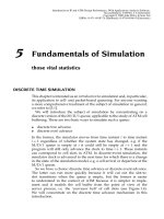
Figure 12.1. Overall Cell Loss Probability against Buffer Capacity for N VBR Sources
COMBINING THE BURST AND CELL SCALES 189
cell-scale queueing component, CLP
cs
, and the burst-scale delay factor,
CLP
bsd
, varying with buffer capacity.
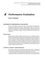
The combined results are plotted in Figure 12.1. The cell-scale compo-
nent is obtained using the exact analysis of the finite M/D/1 described
in Chapter 7. The burst-scale delay factor uses the same approach as that
for calculating the values in Figure 9.16. For Figure 12.1, an average burst
length, b, of 480 cells is used. The overall cell loss shown in Figure 12.1 is
calculated by summing the burst- and cell-scale components of cell loss,
where the burst-scale component is the product of the loss and delay
factors, i.e.
CLP D CLP
cs
C CLP
bsl
Ð CLP
bsd

Now, consider N CBR sources where each source has a constant cell rate
of 2000 cell/s. Figure 12.2 shows how the cell loss varies with the buffer
0102030405060708090100
Buffer capacity, X
Cell loss probability
N = 170
N = 150
N = 120
10
0
10
−1
10
−2
10
−3
10
−4
10
−5
10
−6
10
−7
10
−8
10
−9
10
−10

k:D 0 50
x
k
:D k
y1
k
:D NDD1Q

k , 170 ,
170 Ð 2000
353207. 5

y2
k
:D NDD1Q

k , 150 ,
150 Ð 2000
353207. 5

y3
k
:D NDD1Q

k , 120 ,
120 Ð 2000
353207. 5

Figure 12.2. Cell Loss Probability against Buffer Capacity for N CBR Sources
190 DIMENSIONING

0 102030405060708090100
Buffer capacity, X
10
−10
10
−9
10
−8
10
−7
10
−6
10
−5
10
−4
10
−3
10
−2
10
−1
10
0
Cell loss probability
load = 0.96
load = 0.85
load = 0.68
k:D 0 100
aP68

k
:D Poisson k , 0 . 68
aP85
k
:D Poisson k , 0 . 85
aP96
k
:D Poisson k , 0 . 96
i:D 2 100
x
i
:D i
y1
i
:D finiteQloss x
i
, aP68 , 0 . 68
y2
i
:D finiteQloss x
i
, aP85 , 0 . 85
y3
i
:D finiteQloss x
i
, aP96 , 0 . 96
Figure 12.3. Cell Loss Probability against Buffer Capacity for Random Traffic
capacity for 120, 150 and 170 sources. The corresponding values for the
offered load are 0.68, 0.85, and 0.96 respectively. Figure 12.3 takes the load

values used for the CBR traffic and assumes that the trafficisrandom.
The cell loss results are found using the exact analysis for the finite
M/D/1 system. A summary of the three different situations is depicted
in Figure 12.4, comparing 30 VBR sources, 150 CBR sources, and an
offered load of 0.85 of random traffic (the same load as 150 CBR sources).
DIMENSIONING THE BUFFER
Figure 12.4 shows three very different curves, depending on the charac-
teristics of each different type of source. There is no question that the
DIMENSIONING THE BUFFER 191
0 102030405060708090100
Buffer capacity, X
Cell loss probability
VBR
random
CBR
10
0
10
−1
10
−2
10
−3
10
−4
10
−5
10
−6
10

−7
10
−8
10
−9
10
−10
k:D 0 100
aP85
k
:D Poisson k , 0 . 85
i:D 2 100
x
i
:D i
y1
i
:D NDD1Q

i , 150 ,
150 Ð 2000
353207. 5

y2
i
:D finiteQloss x
i
, aP85 , 0 . 85
y3
i

:D OverallCLP i , 30 , 2000 , 24000 , 353207. 5 , 480
Figure 12.4. Comparison of VBR, CBR and Random TrafficthroughaFiniteBuffer
buffer must be able to cope with the cell-scale component of queueing
since this is always present when a number of traffic streams are merged.
But we have two options when it comes to the burst-scale component, as
analysed in Chapter 9:
1. Restrict the number of bursty sources so that the total input rate only
rarely exceeds the cell slot rate, and assume that all excess-rate cells
are lost. This is the bufferless or burst-scale loss option (also known
as ‘rate envelope multiplexing’).
2. Assume that we have a big enough buffer to cope with excess-
rate cells, so only a proportion are lost; the other excess-rate cells are
delayed in the buffer. This is the burst-scale delay option (rate-sharing
statistical multiplexing).
192 DIMENSIONING
It is important to notice that how big we make the buffer depends on
how we intend to accept traffic onto the network (or vice versa). Also a
dimensioning choice has an impact on a control mechanism (connection
admission control).
For the first option, the buffer is dimensioned according to cell-scale
constraints. The amount of bursty traffic is not the limiting factor in
choosing the buffer capacity because the CAC restrictions on accepting
bursty traffic automatically limit the burst-scale component to a value
below the CLP requirement, and the CAC algorithm assumes that the
buffer size makes no difference. Thus for bursty traffic the mean utiliza-
tion is low and the gradient of its cell-scale component is steep (see
Figure 12.1). However, for either constant-bit-rate or random trafficthe
cell-scale component is much more significant (there is no burst-scale
component), and it is a realistic maximum load of this traffic that deter-
mines the buffer capacity. The limiting factor here is the delay through

the buffer, particularly for interactive services.
If we choose the second option, the amount of bursty trafficcanbe
increased to the same levels of utilization as for either constant-bit-rate
or random traffic – the price to pay is in the size of the buffer which
must be significantly larger. The disadvantage with buffering the excess
(burst-scale) cells is that the delay through a large buffer can be too
great for services like telephony and interactive video, which negates
the aims of having an integrated approach to all telecommunications
services. There are ways around the problem – segregation of traffic
through separate buffers and the use of time priority servers – but this
does introduce further complexity into the network, see Figure 12.5.
We will look at traffic segregation and priorities in more detail in
Chapter 13.


Long Buffer
Single
server
A time priority scheme would involve serving cells
in the short buffer before cells in the long buffer
Short buffer
Delay
sensitive
cells
Loss
sensitive
cells
Figure 12.5. Time Priorities and Segregation of Traffic
DIMENSIONING THE BUFFER 193
Small buffers for cell-scale queueing

A comparison of random trafficandCBRtraffic (see Figure 12.4) shows
that the ‘cell-scale component’ of the random traffic gives a worse CLP
for the same load. Even with 1000 CBR sources, each of 300 cell/s (to
keep the load constant at 0.85), Table 10.3(b) shows that the cell loss is
about 10
9
for a buffer capacity of 50 cells. This is a factor of 10 lower
than for random trafficthroughthesamesizebuffer.
So, to dimension buffers for cell-scale queueing we use a realistic
maximum load of random traffic. Table 12.2 uses the exact analysis for
Table 12.2
buffer
155.52 Mbit/s link 622.08 Mbit/s link
capacity mean maximum mean maximum
load (cells) delay µs delay µs delay µs delay µs
(a) Buffer Dimensioning for Cell-Scale Queueing: Buffer Capacity, Mean and Maximum
Delay, Given the Offered Load and a Cell Loss Probability of 10
8
0.50 16 4.2 45.3 1.1 11.3
0.51 16 4.3 45.3 1.1 11.3
0.52 17 4.4 48.1 1.1 12.0
0.53 17 4.4 48.1 1.1 12.0
0.54 17 4.5 48.1 1.1 12.0
0.55 18 4.6 51.0 1.1 12.7
0.56 18 4.6 51.0 1.2 12.7
0.57 19 4.7 53.8 1.2 13.4
0.58 19 4.8 53.8 1.2 13.4
0.59 20 4.9 56.6 1.2 14.2
0.60 20 5.0 56.6 1.2 14.2
0.61 21 5.0 59.5 1.3 14.9

0.62 21 5.1 59.5 1.3 14.9
0.63 22 5.2 62.3 1.3 15.6
0.64 23 5.3 65.1 1.3 16.3
0.65 23 5.5 65.1 1.4 16.3
0.66 24 5.6 67.9 1.4 17.0
0.67 25 5.7 70.8 1.4 17.7
0.68 25 5.8 70.8 1.5 17.7
0.69 26 6.0 73.6 1.5 18.4
0.70 27 6.1 76.4 1.5 19.1
0.71 28 6.3 79.3 1.6 19.8
0.72 29 6.5 82.1 1.6 20.5
0.73 30 6.7 84.9 1.7 21.2
0.74 31 6.9 87.8 1.7 21.9
0.75 33 7.1 93.4 1.8 23.4
0.76 34 7.3 96.3 1.8 24.1
0.77 35 7.6 99.1 1.9 24.8
(continued overleaf )
194 DIMENSIONING
Table 12.2. (continued)
buffer
155.52 Mbit/s link 622.08 Mbit/s link
capacity mean maximum mean maximum
load (cells) delay µs delay µs delay µs delay µs
0.78 37 7.9 104.8 2.0 26.2
0.79 39 8.2 110.4 2.0 27.6
0.80 41 8.5 116.1 2.1 29.0
0.81 43 8.9 121.7 2.2 30.4
0.82 45 9.3 127.4 2.3 31.9
0.83 48 9.7 135.9 2.4 34.0
0.84 51 10.3 144.4 2.6 36.1

0.85 54 10.9 152.9 2.7 38.2
0.86 58 11.5 164.2 2.9 41.1
0.87 62 12.3 175.5 3.1 43.9
0.88 67 13.2 189.7 3.3 47.4
0.89 73 14.3 206.7 3.6 51.7
0.90 79 15.6 223.7 3.9 55.9
0.91 88 17.1 249.1 4.3 62.3
0.92 98 19.1 277.5 4.8 69.4
0.93 112 21.6 317.1 5.4 79.3
0.94 129 25.0 365.2 6.3 91.3
0.95 153 29.7 433.2 7.4 108.3
0.96 189 36.8 535.1 9.2 133.8
0.97 248 48.6 702.1 12.2 175.5
0.98 362 72.2 1024.9 18.0 256.2
(b) Buffer Dimensioning for Cell-Scale Queueing: Buffer Capacity, Mean and Maximum
Delay, Given the Offered Load and a Cell Loss Probability of 10
10
0.50 19 4.2 53.8 1.1 13.4
0.51 20 4.3 56.6 1.1 14.2
0.52 20 4.4 56.6 1.1 14.2
0.53 21 4.4 59.5 1.1 14.9
0.54 21 4.5 59.5 1.1 14.9
0.55 22 4.6 62.3 1.1 15.6
0.56 23 4.6 65.1 1.2 16.3
0.57 23 4.7 65.1 1.2 16.3
0.58 24 4.8 67.9 1.2 17.0
0.59 24 4.9 67.9 1.2 17.0
0.60 25 5.0 70.8 1.2 17.7
0.61 26 5.0 73.6 1.3 18.4
0.62 26 5.1 73.6 1.3 18.4

0.63 27 5.2 76.4 1.3 19.1
0.64 28 5.3 79.3 1.3 19.8
0.65 29 5.5 82.1 1.4 20.5
0.66 30 5.6 84.9 1.4 21.2
0.67 31 5.7 87.8 1.4 21.9
0.68 32 5.8 90.6 1.5 22.6
0.69 33 6.0 93.4 1.5 23.4
DIMENSIONING THE BUFFER 195
Table 12.2. (continued)
buffer
155.52 Mbit/s link 622.08 Mbit/s link
capacity mean maximum mean maximum
load (cells) delay µs delay µs delay µs delay µs
0.70 34 6.1 96.3 1.5 24.1
0.71 35 6.3 99.1 1.6 24.8
0.72 37 6.5 104.8 1.6 26.2
0.73 38 6.7 107.6 1.7 26.9
0.74 39 6.9 110.4 1.7 27.6
0.75 41 7.1 116.1 1.8 29.0
0.76 43 7.3 121.7 1.8 30.4
0.77 45 7.6 127.4 1.9 31.9
0.78 47 7.9 133.1 2.0 33.3
0.79 49 8.2 138.7 2.0 34.7
0.80 51 8.5 144.4 2.1 36.1
0.81 54 8.9 152.9 2.2 38.2
0.82 57 9.3 161.4 2.3 40.3
0.83 60 9.7 169.9 2.4 42.5
0.84 64 10.3 181.2 2.6 45.3
0.85 68 10.9 192.5 2.7 48.1
0.86 73 11.5 206.7 2.9 51.7

0.87 79 12.3 223.7 3.1 55.9
0.88 85 13.2 240.7 3.3 60.2
0.89 93 14.3 263.3 3.6 65.8
0.90 102 15.6 288.8 3.9 72.2
0.91 113 17.1 319.9 4.3 80.0
0.92 126 19.1 356.7 4.8 89.2
0.93 144 21.6 407.7 5.4 101.9
0.94 167 25.0 472.8 6.3 118.2
0.95 199 29.7 563.4 7.4 140.9
0.96 246 36.8 696.5 9.2 174.1
0.97 324 48.6 917.3 12.2 229.3
0.98 476 72.2 1347.6 18.0 336.9
(c) Buffer Dimensioning for Cell-Scale Queueing: Buffer Capacity, Mean and Maximum
Delay, Given the Offered Load and a Cell Loss Probability of 10
12
0.50 23 4.2 65.1 1.1 16.3
0.51 24 4.3 67.9 1.1 17.0
0.52 24 4.4 67.9 1.1 17.0
0.53 25 4.4 70.8 1.1 17.7
0.54 26 4.5 73.6 1.1 18.4
0.55 26 4.6 73.6 1.1 18.4
0.56 27 4.6 76.4 1.2 19.1
0.57 28 4.7 79.3 1.2 19.8
0.58 28 4.8 79.3 1.2 19.8
0.59 29 4.9 82.1 1.2 20.5
0.60 30 5.0 84.9 1.2 21.2
0.61 31 5.0 87.8 1.3 21.9
(continued overleaf )
196 DIMENSIONING
Table 12.2. (continued)

buffer
155.52 Mbit/s link 622.08 Mbit/s link
capacity mean maximum mean maximum
load (cells) delay µs delay µs delay µs delay µs
0.62 32 5.1 90.6 1.3 22.6
0.63 33 5.2 93.4 1.3 23.4
0.64 34 5.3 96.3 1.3 24.1
0.65 35 5.5 99.1 1.4 24.8
0.66 36 5.6 101.9 1.4 25.5
0.67 37 5.7 104.8 1.4 26.2
0.68 38 5.8 107.6 1.5 26.9
0.69 39 6.0 110.4 1.5 27.6
0.70 41 6.1 116.1 1.5 29.0
0.71 42 6.3 118.9 1.6 29.7
0.72 44 6.5 124.6 1.6 31.1
0.73 46 6.7 130.2 1.7 32.6
0.74 47 6.9 133.1 1.7 33.3
0.75 49 7.1 138.7 1.8 34.7
0.76 52 7.3 147.2 1.8 36.8
0.77 54 7.6 152.9 1.9 38.2
0.78 56 7.9 158.5 2.0 39.6
0.79 59 8.2 167.0 2.0 41.8
0.80 62 8.5 175.5 2.1 43.9
0.81 65 8.9 184.0 2.2 46.0
0.82 69 9.3 195.4 2.3 48.8
0.83 73 9.7 206.7 2.4 51.7
0.84 78 10.3 220.8 2.6 55.2
0.85 83 10.9 235.0 2.7 58.7
0.86 89 11.5 252.0 2.9 63.0
0.87 96 12.3 271.8 3.1 67.9

0.88 104 13.2 294.4 3.3 73.6
0.89 113 14.3 319.9 3.6 80.0
0.90 124 15.6 351.1 3.9 87.8
0.91 138 17.1 390.7 4.3 97.7
0.92 154 19.1 436.0 4.8 109.0
0.93 176 21.6 498.3 5.4 124.6
0.94 204 25.0 577.6 6.3 144.4
0.95 244 29.7 690.8 7.4 172.7
0.96 303 36.8 857.9 9.2 214.5
0.97 400 48.6 1132.5 12.2 283.1
0.98 592 72.2 1676.1 18.0 419.0
the finite M/D/1 queue to show the buffer capacity for a given load and
cell loss probability. The first column is the load, varying from 50% up to
98%, and the second column gives the buffer size for a particular cell loss
probability requirement (Table 12.2 part (a) is for a CLP of 10
8
,part(b)
is for 10
10
,andpart(c)isfor10
12
). Then there are extra columns which
DIMENSIONING THE BUFFER 197
give the mean delay and maximum delay through the buffer for link
rates of 155.52 Mbit/s and 622.08 Mbit/s. The maximum delay is just the
buffer capacity multiplied by the time per cell slot, s, at the appropriate
link rate. The mean delay depends on the load, , and is calculated using
the formula for an infinite M/D/1 system:
t
q

D s C
 Ð s
2 Ð 1  
This is very close to the mean delay through a finite M/D/1 because the
loss is extremely low (mean delays only differ noticeably when the loss
from the finite system is high).
Figure 12.6 presents the mean and maximum delay values from
Table 12.2 in the form of a graph and clearly shows how the delays
increase substantially above a load of about 80%. This graph can be used
to select a maximum load according to the cell loss and delay constraints,
and the buffer’s link rate; the required buffer size can then be read from
the appropriate part of Table 12.2.
So, to summarize, we dimension short buffers to cope with cell-scale
queueing behaviour using Table 12.2 and Figure 12.6. This approach is
applicable to networks which offer the deterministic bit-rate transfer
capability and the statistical bit-rate transfer capability based on rate
envelope multiplexing. For SBR based on rate sharing, buffer dimen-
sioning requires a different approach, based on the burst-scale queueing
behaviour.
0
100
200
300
400
500
600
700
800
900
1000

0.5 0.6 0.7 0.8 0.9 1
Load
Delay in microseconds through
155.52 Mbit/s link buffer
0
25
50
75
100
125
150
175
200
225
250
CLP = 10
−12
CLP = 10
−10
CLP = 10
−8
Delay in microseconds through
622.08 Mbit/s link buffer
Mean delay
Maximum delay
Figure 12.6. Mean and Maximum Delays for a Buffer with Link Rate of either
155.52 Mbit/s or 622.08 Mbit/s for Cell Loss Probabilities of 10
8
,10
10

and 10
12
198 DIMENSIONING
Large buffers for burst-scale queueing
A buffer-dimensioning method for large buffers and burst-scale queueing
is rather more complicated than for short buffers and cell-scale queueing
because the traffic characterization has more parameters. For the cell-
scale queueing case, random traffic is a very good upper bound and it has
just the one parameter: arrival rate. In the burst-scale queueing case, we
must assume a traffic mix of many on/off sources, each source having the
same traffic characteristics (peak cell rate, mean cell rate, and the mean
burst length in the active state). For the burst-scale analytical approach
we described in Chapter 9, the key parameters are the minimum number
of peak rates required for burst-scale queueing, N
0
,theratioofbuffer
capacity to mean burst length, X/b, the mean load, ,andthecellloss
probability.
We have seen in Chapter 10 that the overall cell loss target can be
obtained by trial and error with tables; combining the burst-scale loss
and burst-scale delay factors from Table 10.4 and Table 10.5 respectively.
Here, we present buffer-dimensioning data in two alternative graphical
forms: the variation of X/b with load for a fixed value of N
0
and different
overall CLP values (Figure 12.7); and the variation of X/b with load for a
fixed overall CLP value and different values of N
0
(Figure 12.8).
To produce a graph like that of Figure 12.7, we take one row from

Table 10.4, for a particular value of N
0
. This gives the cell loss contribu-
tion, CLP
bsl
, from the burst-scale loss factor varying with offered load
1
10
100
1000
10000
0.5 0.6 0.7 0.8 0.9 1.0
Load
X/b, buffer capacity in units of
average burst length
CLP = 10
−12
CLP = 10
−10
CLP = 10
−8
Figure 12.7. Buffer Capacity in Units of Mean Burst Length, Given Load and Cell
Loss Probability, for Traffic with a Peak Cell Rate of 1/100 of the Cell Slot Rate (i.e.
N
0
D 100)
COMBINING THE CONNECTION, BURST AND CELL SCALES 199
1
10
100

1000
0.0 0.1 0.2 0.3 0.4 0.5 0.6 0.7 0.8 0.9 1.0
Load
X/b, buffer capacity in units of
average burst length
N
0
= 10, 20, 100, 200, 700
Figure 12.8. Buffer Capacity in Units of Mean Burst Length, Given Load and the
Ratio of Cell Slot Rate to Peak Cell Rate, for a Cell Loss Probability of 10
10
(Table 12.3). We then need to find the value of X/b which gives a cell
loss contribution, CLP
bsd
, from the burst-scale delay factor, to meet the
overall CLP target. This is found by rearranging the equation
CLP
target
CLP
bsl
D CLP
bsd
D e


N
0
Ð
X
b

Ð
1
3
4ÐC1

to give
X
b
D
4 Ð  C 1
1  
3
Ð
ln

CLP
target
CLP
bsl

N
0
Table 12.3 gives the figures for an overall CLP target of 10
10
,and
Figure 12.7 shows results for three different CLP targets: 10
8
,10
10
and

10
12
. Figure 12.8 shows results for a range of values of N
0
for an overall
CLP target of 10
10
.
Table 12.3. Burst-Scale Parameter Values for N
0
D 100 and a CLP Target of 10
10
CLP
bsl
10
1
10
2
10
3
10
4
10
5
10
6
10
7
10
8

10
9
10
10
load,  0.94 0.87 0.80 0.74 0.69 0.65 0.61 0.58 0.55 0.53
CLP
bsd
10
9
10
8
10
7
10
6
10
5
10
4
10
3
10
2
10
1
10
0
X/b 5064.2 394.2 84.6 31.1 14.7 7.7 4.1 2.1 0.8 0
200 DIMENSIONING
COMBINING THE CONNECTION, BURST AND CELL SCALES

We have seen in Chapter 10 that connection admission control can be
based on a variety of different algorithms. An important grade of service
parameter, in addition to cell loss and cell delay, is the probability of
a connection being blocked. This is very much dependent on the CAC
algorithm and the characteristics of the offered traffic types, and in general
it is a difficult task to evaluate the connection blocking probability.
However, if we restrict the CAC algorithm to one that is based on
limiting the number of connections admitted then we can apply erlang’s
lost call formula to the situation. The service capacity of an ATM link
is effectively being divided into N ‘circuits’.Ifallofthese‘circuits’ are
occupied, then the CAC algorithm will reject any further connection
attempts. It is worth noting that the cell loss and cell delay performance
requirements determine the maximum number of connections that can
be admitted. Thus, for much of the time, the traffic mix will have fewer
connections, and the cell loss and cell delay performance will be rather
better than that specified in the trafficcontractrequirements.
Consider the situation with constant-bit-rate traffic. Figure 12.9 plots
the cell loss from a buffer of capacity 10 cells, for a range of CBR sources
where D is the number of slots between arrivals. Thus, with a particular
CLP requirement, and a constant cell rate given by
h D
C
D
cell/s
D=20
D=40
D=60
D=80
D=100
D=150

D=200
D=300
1E−12
1E−11
1E−10
1E−09
1E−08
1E−07
1E−06
1E−05
1E−04
1E−03
1E−02
1E−01
1E+00
0102030
40
50 60 70 80 90 100
Maximum number of connections
Cell loss probability
Figure 12.9. Maximum Number of CBR Connections, Given D Cell Slots between
Arrivals and CLP
COMBINING THE CONNECTION, BURST AND CELL SCALES 201
(where C is the cell slot rate), we can find from Figure 12.9 the maximum
number of connections that can be admitted onto a link of cell rate C.
The link cannot be loaded to more than 100% capacity, so the maximum
possible number of sources of any particular type is numerically equal
to the (constant) number of cell slots between arrivals. Let’stakean
example. Suppose we have CBR sources of cell rate 3532 cell/s being
multiplexed over a 155.52 Mbit/s link, with a CLP requirement of 10

7
.
This gives a value of 100 for D, and from Figure 12.9, the maximum
number of connections is (near enough) 50.
Now that we have a figure for the maximum number of connections,
we can calculate the offered traffic at the connection level for a given
probability of blocking. Figure 12.10 shows how the connection blocking
probability varies with the maximum number of connections for different
offered traffic intensities. With our example, we find that for 50 connec-
tions maximum and a connection blocking probability of 0.02, the offered
traffic intensity is 40 erlangs. Note that the mean number of connections
in progress is numerically equal to the offered traffic, i.e. 40 connections.
The cell loss probability for this number of connections can be found
from Figure 12.9: it is 2 ð 10
9
.Thisisoveranorderofmagnitudelower
than the CLP requirement in the traffic contract, and therefore provides
a useful safety margin.
For variable-bit-rate traffic, we will only consider rate envelope multi-
plexing and not rate sharing. Figure 12.11 shows how the cell loss
20 E 30 E 40 E 50 E 60 E10 E
70 E
80 E
90 E
100 E
0.0001
0.001
0.01
0.1
1

0 102030405060708090100
Maximum number of connections
Probability of connection blocking
Figure 12.10. Probability of Blocking, Given Maximum Number of Connections and
Offered Traffic
202 DIMENSIONING
1E−12
1E−11
1E−10
1E−09
1E−08
1E−07
1E−06
1E−05
1E−04
1E−03
1E−02
1E−01
1E+00
0 0.1 0.2 0.3 0.4 0.5 0.6 0.7 0.8 0.9 1
Load
Cell loss probability
N
0
=10, 20, 100
Figure 12.11. Maximum Utilization for VBR Connections, Given N
0
and CLP
probability from a (short) buffer varies with the utilization for a range of
VBR sources of different peak cell rates. The key parameter defining this

relationship is N
0
, the ratio of the cell slot rate to the peak cell rate. Given
N
0
and a CLP requirement, we can read off a value for the utilization.
This then needs to be multiplied by the ratio of the cell slot rate, C,tothe
mean cell rate, m, to obtain the maximum number of connections that can
be admitted onto the link.
So, for example, for sources with a peak cell rate of 8830 cell/s and
a mean cell rate of 3532 cell/s being multiplexed onto a 155.52 Mbit/s
link, N
0
is 40 and, according to Figure 12.11, the utilization is about
0.4foraCLPof10
8
. This utilization is multiplied by 100 (i.e. C/m)
to give a maximum of 40 connections. From Figure 12.10, an offered
traffic intensity of 30 erlangs gives a connection blocking probability of
just under 0.02 for 40 connections maximum. Thus the mean number
of connections in progress is 30, giving a mean load of 0.3, and from
Figure 12.11 the corresponding cell loss probability is found to be 10
11
.
This is three orders of magnitude better than for the maximum number
of connections.
As an alternative to using Figure 12.10, a traffic table based on Erlang’s
lost call formula is provided in Table 12.4.
So,wehaveseenthat,forbothCBRandVBRtraffic, when the connec-
tion blocking probability requirements are taken into account, the actual

cell loss probability can be rather lower than that for the maximum
allowed number of connections.
COMBINING THE CONNECTION, BURST AND CELL SCALES 203
Table 12.4. Traffic Table Based on Erlang’s Lost Call Formula
Probability of blocking a connection
N 0.1 0.05 0.02 0.01 0.005 0.001 0.0001
offered traffic in erlangs:
1 0.11 0.05 0.02 0.01 0.005 0.001 0.0001
2 0.59 0.38 0.22 0.15 0.10 0.04 0.03
3 1.27 0.89 0.60 0.45 0.34 0.19 0.08
4 2.04 1.52 1.09 0.86 0.70 0.43 0.23
5 2.88 2.21 1.65 1.36 1.13 0.76 0.45
6 3.75 2.96 2.27 1.90 1.62 1.14 0.72
7 4.66 3.73 2.93 2.50 2.15 1.57 1.05
8 5.59 4.54 3.62 3.12 2.72 2.05 1.42
9 6.54 5.37 4.34 3.78 3.33 2.55 1.82
10 7.51 6.21 5.08 4.46 3.96 3.09 2.26
11 8.48 7.07 5.84 5.15 4.61 3.65 2.72
12 9.47 7.95 6.61 5.87 5.27 4.23 3.20
13 10.46 8.83 7.40 6.60 5.96 4.83 3.71
14 11.47 9.72 8.20 7.35 6.66 5.44 4.23
15 12.48 10.63 9.00 8.10 7.37 6.07 4.78
16 13.50 11.54 9.82 8.87 8.09 6.72 5.33
17 14.52 12.46 10.65 9.65 8.83 7.37 5.91
18 15.54 13.38 11.49 10.43 9.57 8.04 6.49
19 16.57 14.31 12.33 11.23 10.33 8.72 7.09
20 17.61 15.24 13.18 12.03 11.09 9.41 7.70
21 18.65 16.18 14.03 12.83 11.85 10.10 8.31
22 19.69 17.13 14.89 13.65 12.63 10.81 8.94
23 20.73 18.07 15.76 14.47 13.41 11.52 9.58

24 21.78 19.03 16.63 15.29 14.20 12.24 10.22
25 22.83 19.98 17.50 16.12 14.99 12.96 10.88
26 23.88 20.94 18.38 16.95 15.79 13.70 11.53
27 24.93 21.90 19.26 17.79 16.59 14.43 12.20
28 25.99 22.86 20.15 18.64 17.40 15.18 12.88
29 27.05 23.83 21.03 19.48 18.21 15.93 13.56
30 28.11 24.80 21.93 20.33 19.03 16.68 14.24
31 29.17 25.77 22.82 21.19 19.85 17.44 14.93
32 30.23 26.74 23.72 22.04 20.67 18.20 15.63
33 31.30 27.72 24.62 22.90 21.50 18.97 16.33
34 32.36 28.69 25.52 23.77 22.33 19.74 17.04
35 33.43 29.67 26.43 24.63 23.16 20.51 17.75
36 34.50 30.65 27.34 25.50 24.00 21.29 18.46
37 35.57 31.63 28.25 26.37 24.84 22.07 19.18
38 36.64 32.62 29.16 27.25 25.68 22.86 19.91
39 37.71 33.60 30.08 28.12 26.53 23.65 20.63
40 38.78 34.59 30.99 29.00 27.38 24.44 21.37
(continued overleaf )
204 DIMENSIONING
Table 12.4. (continued)
Probability of blocking a connection
N 0.1 0.05 0.02 0.01 0.005 0.001 0.0001
offered traffic in erlangs:
41 39.86 35.58 31.91 29.88 28.23 25.23 22.10
42 40.93 36.57 32.83 30.77 29.08 26.03 22.84
43 42.01 37.56 33.75 31.65 29.93 26.83 23.58
44 43.08 38.55 34.68 32.54 30.79 27.64 24.33
45 44.16 39.55 35.60 33.43 31.65 28.44 25.08
46 45.24 40.54 36.53 34.32 32.51 29.25 25.83
47 46.32 41.54 37.46 35.21 33.38 30.06 26.58

48 47.40 42.53 38.39 36.10 34.24 30.87 27.34
49 48.48 43.53 39.32 37.00 35.11 31.69 28.10
50 49.56 44.53 40.25 37.90 35.98 32.51 28.86
55 54.9 49.5 44.9 42.4 40.3 36.6 32.7
60 60.4 54.5 49.6 46.9 44.7 40.7 36.6
65 65.8 59.6 54.3 51.5 49.1 44.9 40.5
70 71.2 64.6 59.1 56.1 53.6 49.2 44.5
75 76.7 69.7 63.9 60.7 58.1 53.5 48.6
80 82.2 74.8 68.6 65.3 62.6 57.8 52.6
85 87.6 79.9 73.4 70.0 67.2 62.1 56.7
90 93.1 85.0 78.3 74.6 71.7 66.4 60.9
95 98.6 90.1 83.1 79.3 76.3 70.8 65.0
100 104.1 95.2 87.9 84.0 80.9 75.2 69.2
105 109.5 100.3 92.8 88.7 85.5 79.6 73.4
110 115.0 105.4 97.6 93.4 90.1 84.0 77.6
115 120.5 110.6 102.5 98.2 94.7 88.5 81.9
120 126.0 115.7 107.4 102.9 99.3 92.9 86.2
125 131.5 120.9 112.3 107.7 104.0 97.4 90.4
130 137.0 126.0 117.1 112.4 108.6 101.9 94.7
135 142.5 131.2 122.0 117.2 113.3 106.4 99.0
140 148.1 136.3 126.9 122.0 118.0 110.9 103.4
145 153.6 141.5 131.8 126.7 122.7 115.4 107.7
150 159.1 146.7 136.8 131.5 127.3 119.9 112.1
155 164.6 151.8 141.7 136.3 132.0 124.4 116.4
160 170.1 157.0 146.6 141.1 136.7 129.0 120.8
165 175.6 162.2 151.5 145.9 141.5 133.5 125.2
170 181.1 167.3 156.4 150.7 146.2 138.1 129.6
175 186.7 172.5 161.4 155.5 150.9 142.6 134.0
180 192.2 177.7 166.3 160.4 155.6 147.2 138.4
185 197.7 182.9 171.3 165.2 160.4 151.8 142.8

190 203.2 188.1 176.2 170.0 165.1 156.4 147.2
195 208.7 193.3 181.2 174.9 169.8 161.0 151.7
200 214.0 198.5 186.1 179.7 174.6 165.6 156.1