Comparing receptor binding properties of 2019 ncov virus with those of sars cov virus using computational biophysics approach
Bạn đang xem bản rút gọn của tài liệu. Xem và tải ngay bản đầy đủ của tài liệu tại đây (10.38 MB, 48 trang )
VIETNAM NATIONAL UNIVERSITY, HANOI
VIETNAM JAPAN UNIVERSITY
CONG PHUONG CAO
COMPARING RECEPTOR BINDING
PROPERTIES OF 2019-nCoV VIRUS WITH
THOSE OF SARS-CoV VIRUS USING
COMPUTATIONAL BIOPHYSICS
APPROACH
MASTER'S THESIS
VIETNAM NATIONAL UNIVERSITY, HANOI
VIETNAM JAPAN UNIVERSITY
CONG PHUONG CAO
COMPARING RECEPTOR BINDING
PROPERTIES OF 2019-nCoV VIRUS WITH
THOSE OF SARS-CoV VIRUS USING
COMPUTATIONAL BIOPHYSICS APPROACH
MAJOR: NANOTECHNOLOGY
CODE: 8440140.11 QTD
RESEARCH SUPERVISOR:
Associate Prof. Dr. NGUYEN THE TOAN
Hanoi, 2021
Acknowledgements
It could be said that without Prof. Nguyen The Toan, I couldn’t have gone this far in my
scientific research path, much less conducting this master thesis. Therefore, first of all, I
want to express my sincere thank to Prof. Nguyen The Toan as my beloved master thesis
supervisor in the VNU Key Laboratory on Multiscale Simulation of Complex Systems
and the Faculty of Physics, VNU University of Science, Vietnam National University.
I also wish to thank Dr. Pham Trong Lam, who guided me in my very first steps in the
machine learning field as well as give me precious advice for my research during my
internship period and thesis defense preparation.
I would like to thank the lecturers in VJU Master’s Program in Nanotechnology for many
inspirational discussions and helpful knowledge from classes.
I would also like to thank all staff, lecturers, and my good friends in VJU for helping me
a lot during my memorable study in VJU.
This research is funded by Vietnam National University under grant number QG.20.82.
Hanoi, 17 July 2021
Cong Phuong Cao
Contents
Acknowledgements
i
List of Tables
iv
List of Figures
v
List of Abbreviations
vi
1
INTRODUCTION
1
2
MOLECULAR DYNAMICS SIMULATION
2.1 Molecular Dynamics . . . . . . . . . . .
2.1.1 Integration Algorithm . . . . . .
2.1.2 Force field . . . . . . . . . . . .
2.2 Materials and Models . . . . . . . . . . .
2.3 Simulation Details . . . . . . . . . . . .
2.3.1 Thermostat and Barostat . . . . .
2.3.2 Periodic Boundary Conditions . .
3
4
ANALYSES METHODS
3.1 Sequence Alignment . . . . .
3.2 Root Mean Square Deviation .
3.3 Root Mean Square Fluctuation
3.4 Principal Component Analysis
3.5 Variational Autoencoder . . .
.
.
.
.
.
.
.
.
.
.
.
.
.
.
.
.
.
.
.
.
.
.
.
.
.
.
.
.
.
.
.
.
.
.
.
.
.
.
.
.
.
.
.
.
.
.
.
.
.
.
.
.
.
.
.
.
.
.
.
.
.
.
.
.
.
.
.
.
.
.
.
.
.
.
.
.
.
.
.
.
.
.
.
.
.
.
.
.
.
.
.
.
.
.
.
.
.
.
.
.
.
.
.
.
.
.
.
.
.
.
.
.
.
.
.
.
.
.
.
.
.
.
.
.
.
.
.
.
.
.
.
.
.
.
.
.
.
.
.
.
.
.
.
.
.
.
.
.
.
.
.
.
.
.
.
.
.
.
.
.
.
.
.
.
.
.
.
.
.
.
.
.
.
.
RESULTS AND DISCUSSION
4.1 Preliminary Sequence Alignments of The Viral RBDs . . . . . .
4.2 Deviations and Fluctuations of The Structural Backbone Atoms .
4.2.1 Root Mean Square Deviations . . . . . . . . . . . . . .
4.2.2 Root Mean Square Fluctuations . . . . . . . . . . . . .
4.3 Principal Component Analysis . . . . . . . . . . . . . . . . . .
4.4 Machine Learning on 6M0J System . . . . . . . . . . . . . . .
.
.
.
.
.
.
.
.
.
.
.
.
.
.
.
.
.
.
.
.
.
.
.
.
.
.
.
.
.
.
.
.
.
.
.
.
.
.
.
.
.
.
.
.
.
.
.
.
.
.
.
.
.
.
.
.
.
.
.
.
.
4
4
5
6
8
9
9
10
.
.
.
.
.
13
13
13
14
14
15
.
.
.
.
.
.
19
19
20
21
22
25
27
CONCLUSIONS
30
REFERENCES
32
ii
A IN-HOUSE SOURCE CODE
A.1 Data Pre-processing Source Code . . . . . . . . . . . . . . . . . . . .
A.2 Autoencoder Source Code . . . . . . . . . . . . . . . . . . . . . . . .
35
35
35
B ADDITIONAL VAE RESULTS
38
iii
List of Tables
2.1
The molecules simulated for each systems. . . . . . . . . . . . . . . . .
9
3.1
The detailed parameters of VAE model. . . . . . . . . . . . . . . . . .
18
4.1
The trace of the co-variance matrix of the projections of the protein
backbones on the two largest principal components. . . . . . . . . . . .
26
iv
List of Figures
1.1
1.2
2.1
The binding of coronavirus spike protein to human ACE2 receptor . . .
Antibodies neutralizing SARS-CoV-2 virus by blocking its interaction
with human ACE2 receptor. . . . . . . . . . . . . . . . . . . . . . . . .
2
3
A 2-dimensional PBC view along the z-axis direction of the 6VW1 system. The primitive system is surrounded and interacts with its images. .
A typical snapshot of the 6M0J system after being simulated for 800ns
showing the arrangement of RBD and ACE2 fluctuating in water. . . . .
12
3.1
Illustration of VAE structure used for protein datasets. . . . . . . . . . .
16
4.1
The sequence alignments of the viral RBD of 6VW1 and 6M0J for two
variants of SARS-CoV-2 virus, and of 2AJF for SARS-CoV virus . . .
The location of four discovered significant mutations of the viral RBD .
The root mean square deviations of the backbone of the human ACE2
receptor and of the viral RBD protein. . . . . . . . . . . . . . . . . . .
The root mean square fluctuations of the backbone of the human ACE2
receptor and of the viral RBD protein. . . . . . . . . . . . . . . . . . .
The location of residue 113 of the viral RBD in the 6VW1 system . . .
The location of residue 50 of the viral RBD in the 2AJF system . . . . .
The probability density in the plane of the two largest principal components from the PCA of the backbones structure of proteins . . . . . . .
Latent space projection of variational autoencoder trained on the distance matrix of RBD-ACE2 complex of 6M0J . . . . . . . . . . . . . .
2.2
4.2
4.3
4.4
4.5
4.6
4.7
4.8
B.1 Latent space projection of variational autoencoder
tance matrix of RBD-ACE2 complex of 6M0J . . .
B.2 Latent space projection of variational autoencoder
tance matrix of RBD-ACE2 complex of 6M0J . . .
B.3 Latent space projection of variational autoencoder
tance matrix of RBD-ACE2 complex of 6M0J . . .
trained
. . . .
trained
. . . .
trained
. . . .
on
. .
on
. .
on
. .
the
. .
the
. .
the
. .
dis. . .
dis. . .
dis. . .
11
19
20
21
23
24
25
27
28
38
39
40
v
List of Abbreviations
SARS
SARS-CoV-2
2019-nCoV
SARS-CoV or SARS-CoV-1
RBD
ACE2
MD
EOM
RCSB
PDB
PBC
PME
RMSD
RMSF
PCA
VAE
DAE
Severe Acute Respiratory Syndrome
Severe Acute Respiratory Syndrome CoronaVirus 2
2019 Novel CoronaVirus, colloquial name of SARS-CoV-2
Severe Scute Respiratory Syndrome CoronaVirus
(caused the epidemic in June 2003, different from 2019-nCoV)
Receptor-Binding Domain
Angiotensin Converting Enzyme 2
Molecular Dynamics
Newton’s Equations of Motion
The Research Collaboratory for Structural Bioinformatics
Protein Data Bank
Periodic Boundary Conditions
Particle Mesh Ewald
Root Mean Square Deviation
Root Mean Square Fluctuation
Principal Component Analysis
Variational Autoencoder
Deep Autoencoder
vi
Chapter 1 INTRODUCTION
By the end of 2019, the Severe acute respiratory syndrome coronavirus 2 (SARS-CoV-2)
(also known as 2019-nCoV) was detected in Wuhan city, China, and spread rapidly to
all over the countries and regions, forcing The World Health Organization must declare
a public health emergency only three months later [1]. Because of the extremely fast
spread rate, fast mutation rate and the toxicity of the SARS-CoV-2, scientists are rushing
to find a cure for severe acute respiratory syndrome caused by the virus. It turns out
that the genome of SARS-CoV-2 is very similar to the genome of other coronaviruses
and can be classified as a variant of the Severe acute respiratory syndrome coronavirus
(SARS-CoV), which caused the SARS epidemic in June 2003.
The structure of coronavirus can be divided into two parts, namely core and shell. The
viral core is the single-stranded RNA viral genome. The viral shell is the combination of
fat lipids, envelope proteins, and spike proteins, in which spike proteins play an important role in the entry of the RNA viral genome into the host cell. The receptor-binding
domain (RBD) is a subunit of the spike glycoprotein (also known as protein S) attached
to the viral outer shell [2], [3]. RBD recognizes and binds to human cells through a
receptor call Angiotensin Converting Enzyme 2 (ACE2), like a key being inserted into
a lock (illustrated in Figure 1.1) [4]. After that, the coronavirus is incorporated into the
host cell to release the viral RNA into the cytoplasm.
According to [6]–[10], the RBD of SARS-CoV and SARS-CoV-2 have significant similarities in genome sequence and also use the same cellular entry receptor, namely ACE2.
Because of the critical relation between SARS-CoV and SARS-CoV-2, there raises an
important question: What are the significant differences (mutations) between them making SARS-CoV-2 much more contagious and dangerous? It is supposed that the mutations in the RBD of SARS-CoV-2 in respect of that of SARS-CoV can impact the binding affinity for the ACE2 receptor [8], [11]. In this study, we aimed to answer the above
question by analyzing the structural differences in the binding of RBDs of two variants
of SARS-CoV-2 and SARS-CoV to the human ACE2 receptor.
1
F IGURE 1.1: The binding of coronavirus spike protein to human
ACE2 receptor. (The figure is from [5])
One of the approaches is to study the behavior of the coronaviruses (including SARSCoV-2) interactions with the human ACE2 receptor using computational biophysics approaches, such as molecular dynamics and unsupervised machine learning techniques.
In this study, we use both molecular dynamics and machine learning. To investigate the
characteristics of the binding mechanism of the complex of RBD protein and ACE2 receptor, conventional molecular dynamics is used to simulate the molecular interactions.
The trajectories obtained from the molecular dynamics simulation are then used as input
for the principal component analysis (PCA) and the variational autoencoder (unsupervised learning methods) to extract features (knowledge) of the binding.
It is expected that from knowing the binding mechanism between the viral RBDs and
the ACE2 receptor, one can build and develop antibodies or antiviral drugs based on
the binding features of the RBD of the SARS-CoV-2 spike protein. The SARS-CoV-2
spike protein is the main target for antibodies and antiviral drugs design throughout the
2
vaccine history. Antibodies and some antiviral drugs work on the principle of attacking
the RBD of viruses, binding to RBD regions before the viruses can interact with the
ACE2 receptor (Figure 1.2). By understanding the mechanism between the SARS-CoV2 RBD and the human ACE2 receptor, it is possible to design and develop therapeutic
antibodies and antivirals for the treatment of acute respiratory infections caused by the
virus. Noticeably, not all therapeutic antibodies or antivirals work well with different
viruses of the same strain. This is because of the difference in structure caused by
mutations between virus variants [8], [11]. Therefore, to evaluate the reliability of the
model, we need to study the interaction mechanism of the SARS-CoV-2 coronavirus
with ACE2 in comparison with the interaction mechanism of other coronaviruses.
F IGURE 1.2: Antibodies neutralizing SARS-CoV-2 virus by blocking its interaction with human ACE2 receptor.
This thesis is organized as follows. After Chapter 1 about introduction, the methodology
of the simulation and analyses are described in Chapter 2 and Chapter 3 respectively. All
results are shown and discussed in Chapter 4. And Chapter 4.4 is the conclusions.
3
Chapter 2 MOLECULAR DYNAMICS SIMULATION
2.1
Molecular Dynamics
Molecular dynamics (MD) is a computer simulation technique that is used widely for
theoretical study of many-body systems [12], or in our case of biological systems of
the RBD-ACE2 complex. MD algorithm can calculate the time evolution of the system
based on the given initial configuration (positions and velocities) of the system. In other
words, from an initial configuration of the system, MD can predict the future configurations, which are called trajectory, with some tolerable errors while the behavior of the
system still obeys the ergodic hypothesis in physics and thermodynamics. The trajectory
of the system reveals detailed information on the changes and fluctuations of the proteins
and nucleic acids. As a result, the MD is a very suitable and powerful tool to investigate
the thermodynamics and structure of biological systems, or in our case of the systems of
the RBD-ACE2 complex.
The conventional molecular dynamics method come from the Newton’s second law.
Assume that our system has N particles (atoms), the particle ith has the mass mi , position
ri and acceleration ai = d 2 ri /dt 2 at the current time. Hence, governed by the Newton’s
equations of motion (EOM) the force applied to the particle ith can be expressed as
Fi = mi ai
(2.1)
On the other hand, assume that the interacting potential (potential energy) between particles is known as function of positions ri of N particles, such as U(r1 , r2 , ..., rN ). Hence,
the force applied to the particle ith can be also derived from the derivative (the gradient)
of U(r1 , r2 , ..., rN ) as
Fi = −∇iU(r1 , r2 , ..., rN ) = −
∂U
∂ ri
(2.2)
4
Combining equations 2.1 and 2.2 yields
1 ∂U
d 2 ri
=
−
dt 2
mi ∂ ri
(2.3)
The MD simulation essentially focuses on solving the above equations 2.3 for a period
of time.
2.1.1
Integration Algorithm
The system of equations 2.3 is for the many-body problem. Therefore, there is no analytical solution for the system of equations 2.3. Approximations and numerical solutions are more sensible approaches. Based on the finite difference methods, there are
many numerical algorithms (integrators) are available. Some most famous algorithms
are the Verlet algorithm, Verlet-velocity algorithm, and leap-frog (or leap-frog Verlet)
algorithm.
There are many criteria of an algorithm, such as
• The algorithm should approximate the true trajectory for a long period of time with
some tolerable errors.
• The algorithm should be time-reversible.
• The algorithm should be fast enough to perform.
• The algorithm should be easy to implement.
• The algorithm should conserve some macroscopic physical quantities.
In this thesis, the leap-frog algorithm is chosen for integrating Newton’s EOM. The
reason for this choice is that the leap-frog algorithm satisfies all those criteria and is
good enough to some extent in comparison with other algorithms. Importantly, the leapfrog algorithm is not only fast but also obeys the ergodic hypothesis in physics and
thermodynamics making the physical quantities calculated from system configurations
reliable.
5
Assume that the time-step is ∆t, the position and acceleration vectors of the particle ith
at the current time t are ri (t) and ai (t) respectively. In this algorithm, the velocities
are assumed to be first calculated at the time t − ∆t/2 as vi (t − ∆t/2). The leap-frog
algorithm follows the following scheme:
1. Compute accelerations from the current positions
ai (t) = −
1 ∂U(r1 (t), r2 (t), ..., rN (t))
mi
∂ ri
(2.4)
2. Compute the new velocity at the next half time-step
1
1
vi (t + ∆t) = vi (t − ∆t) + ai (t)∆t
2
2
(2.5)
3. Compute the new position at the next time-step
1
ri (t + ∆t) = ri (t) + vi (t + ∆t)∆t
2
(2.6)
4. Advance to next time step and repeat from step (1)
To calculate the total energy at the time t, the velocities can be approximated by:
vi (t) =
2.1.2
1
1
1
vi (t − ∆t) + vi (t + ∆t)
2
2
2
(2.7)
Force field
In MD simulation, the interacting potential U(r1 , r2 , ..., rN ) that we assumed in equation
2.2 plays an important role in determining the force between particles (atoms). The
interatomic potential of an interacting system can be expanded in terms of many-body
expansion as
U(r1 , ..., rN ) = ∑ U1 (ri )+
i
∑ U2(ri, r j )+ ∑
i, j>i
i, j>i,k> j
U3 (ri , r j , rk )+
∑
U4 (ri , r j , rk , rl )+. . .
i, j>i,k> j,l>k
(2.8)
6
where i, j, k, l are indexes of particles of system, U1 is one-body term showing the external potential acting on a particle, U2 is two-body term showing the interaction between
only two particles, U3 is three-body term showing the interaction between only three
particles, and U4 is four-body term similarly.
For biological systems, there is usually no one-body term as well as expansion 2.8 only
need to truncate at U4 because the larger-than-four-body terms are excessive and needless whereas the other terms are enough to describe the physical picture the system with
a reasonable computational cost. The empirical force fields U are usually used, whose
parameters are obtained from experiments or quantum mechanical calculations. The
force fields U from expansion 2.8 for biological systems typically has the form
U = Evdw + Eelect + Ebonds + Ebends + Edihedrals
(2.9)
where Evdw is van der Waals potential, Eelect is electrostatic potential, Ebonds is bond
distances stretching potential, Ebends is bond angles bending potential, and Edihedrals is
the bond torsion angle potential.
From expression 2.9 , Evdw + Eelect + Ebonds is equivalent to two-body term U2 of expression 2.8. Term Ebends and Edihedrals are equivalent to U3 and U4 respectively. Moreover,
the first two terms of expression 2.9 are considered as non-bonded interactions between
atoms. The last three terms of 2.9 represent the bonded or intramolecular bonding interactions as multiplets of atoms are connected by chemical bonds.
In detail, every terms in 2.9 can be expressed as follow
atoms
Evdw =
∑
i< j
atoms
Eelect =
∑
i< j
Ai j Bi j
− 6
ri12j
ri j
qi q j
4πε0 ri j
1
kr (r − req )2
bonds 2
1
Ebends = ∑ kθ (θ − θeq )2
bends 2
Ebonds =
∑
(2.10)
(2.11)
(2.12)
(2.13)
7
Edihedrals =
1
Vn (1 + cos(nϕ) − γ)
2
dihedrals
∑
(2.14)
In the non-bonded interaction, Lennard-Jones 12-6 potential is usually used to approximate the van der Waals potential term 2.10 with ri j is the distance between atom i and
atom j and parameters Ai j and Bi j are specialized for atomtypes of atom i and j. The
term 2.11 is evaluated when the both charges of atom i and j are not zero but qi and q j
instead. The vacuum permittivity is denoted by ε0 .
In the bonded interactions, the bond stretching and angle bending can be both described
by the harmonic pendulum oscillation model. Therefore, the term 2.12 and 2.13 have
harmonic energy functions where req and θeq are bond lengths constants and angles
constants at equilibrium states, kr and kθ are the vibrational constants. In the bond
torsion angle potential 2.14, the torsional barrier Vn corresponds to the nth barrier for a
particular torsional angle and phase γ.
2.2
Materials and Models
There are two variants of SARS-CoV-2 viruses that are investigated during this work.
The complexes of RBD and ACE2 are obtained from the Research Collaboratory for
Structural Bioinformatics (RCSB) Protein Data Bank (PDB) [13] database with ID:
2AJF [14] for the SARS-CoV virus and 6M0J [15], 6VW1 [16] for two variants of
SARS-CoV-2 viruses. From now on, these systems will be referred to as 2AJF, 6M0J
and 6VW1 respectively for easy identification.
The primary sequences of RBD protein of SARS-CoV virus and SARS-CoV-2 viruses
are aligned using Multiple Sequence Alignment by ClustalW [17] web-server of Kyoto
University Bioinformatics Center with BLOSUM matrix [18].
For the main molecular simulations, the initial simulation configurations of all systems
are generated using CHARMM-GUI web-server [19] and are manually adjusted afterward. The GROMACS/2018.6 software package [20] is used to run MD simulations on
the systems.
8
For the force fields, many force field packages are used depending on the functioning
of each component of the system. The proteins and ions of the system are simulated
using parameters from Charmm-336 force field [21]. For the glycans, a part of ACE2
receptor, GLYCAM06 force field [22] is chosen for the parametrization. The explicit
solvent model TIP3P [23] is applied to represent water in the system. The total charges
of the system are neutralized by adding sodium and chlorine ions. In addition, the physiological salt concentration in the human cell environment is about 150mM determining
the number of added Na+ and Cl- ions. The detailed numbers of molecules of systems
are described in Table 2.1.
TABLE 2.1: The molecules simulated for each systems.
2AJF
6VW1
6M0J
# Residues # Atoms # Residues # Atoms # Residues # Atoms
ACE2
RBD
H2 O
Na+
ClZn2+
597
180
66380
Total
2.3
2.3.1
9673
2848
199140
213
189
1
212064
597
194
87382
9802
3070
262146
275
250
1
275544
597
194
76599
9598
3020
229797
241
218
1
242874
Simulation Details
Thermostat and Barostat
The interactions between the viral RBD and the human ACE2 happen in human body.
Accordingly, the temperature of all systems is also the temperature of the human body
that is 310 K. The pressure of the systems is 1 atm. However, one needs to make the
temperature and pressure behaving naturally as much as possible. In other words, the
systems need to conduct in the correct type of thermodynamics ensembles, which are
characterized by the restraint of some specific thermodynamic quantities. In case of our
systems, isothermal-isobaric (NPT) ensemble describes the realistic systems the best.
To mimic the system in such ensemble, thermostat and barostat algorithms are required
to regulate the temperature and pressure throughout the MD run.
9
In the equilibrating stage of simulation (very early stage), the velocity-rescaling thermostat and Berendsen barostat are implemented to guide the system to the equilibrium
states as fast as possible. These algorithms save a lot of time and computational cost despite the fact that they do not have much physical meaning. Besides, the non-equilibrium
configurations of the system are not of interest. The equilibrating procedure is performed
in 1 ns.
In the MD production run, the Nosé-Hoover thermostat and Parrinello-Rahman barostat
are chosen for the simulations. Both Nosé-Hoover thermostat and Parrinello-Rahman
barostat add an extra degree of freedom to the system to regulate the temperature and
pressure gradually, not abruptly in comparison with velocity-rescaling thermostat and
Berendsen barostat. This is also how the realistic systems behave, making Nosé-Hoover
thermostat and Parrinello-Rahman barostat accurate and efficient methods for isothermalisobaric ensemble MD simulation. The total simulation time of this procedure is 2 µs,
with time-step 2 fs.
2.3.2
Periodic Boundary Conditions
The periodic boundary conditions (PBC) opens the boundary of the system mimicking
the infinite clones of the primitive system which surrounding and interacting with the
primitive system (Figure 2.1). When a component of the system passes through the
boundary of the box, it is put back to the opposite side of the box. This idea is equivalent
to the description that a part of the system lost will be recompensed by the exact part of
another system coming from the opposite direction.
MD simulations are typically run using PBC to reduce boundary effects and simulate
the presence of the bulk environment if the size of the box is big enough. In this work,
the box is cubic with an edge of 14nm to guarantee that the RBD-ACE2 complex and
its periodic complex are far enough, at least 3nm from each other, to prevent unwanted
interactions such as electrostatic screening effect. Because the electrostatic screening
length at 150mM NaCl concentration is around 7Å, this 3nm separation is more than
10
F IGURE 2.1: A 2-dimensional PBC view along the z-axis direction
of the 6VW1 system. The primitive system is surrounded and interacts with its images.
enough to avoid the finite size effect caused by long-range electrostatic interactions between proteins in nearby simulation boxes. To deal with the long-range electrostatic
interaction, Particle Mesh Ewald (PME) method is used with the cutoff length of 1.2nm.
The cutoff length of van der Waals interaction is also 1.2nm.
11
F IGURE 2.2: A typical snapshot of the 6M0J system after being
simulated for 800ns showing the arrangement of RBD and ACE2
fluctuating in water.
12
Chapter 3 ANALYSES METHODS
3.1
Sequence Alignment
Sequence alignment is a method of arranging two or more genome sequences in order
to achieve maximum similarity [24]. These sequences may be interleaved with spaces
at possible locations to form identical or similar columns. The term "sequence alignment" refers to the act of constructing this arrangement, or identifying the best potential
arrangements in a database of unique sequences.
In bioinformatics, this method is often used to study the evolution of sequences from a
common ancestor, especially biological sequences such as protein sequences or DNA,
RNA sequences. Incorrect matches in the sequence correspond to mutations and gaps
correspond to additions or deletions. In this work, the sequence alignment is used for the
viral RBDs of both SARS-CoV virus and SARS-CoV-2 viruses to elucidate the common
features as well as the viral mutations during the time of more than a decade. From the
point of view of a biophysicist, the mutations of SARS-CoV-2 make some considerable
changes in the protein backbone. These changes would make the protein backbone more
rigid/flexible causing significant changes in the way the virus binding to the human
ACE2.
3.2
Root Mean Square Deviation
The root mean square deviation (RMSD) is a common method analyzing the displacement of a group of atoms of a system configuration with respect to a reference system
configuration at a particular time.
Assume that a group of N atoms are examined. Atoms are labeled from 1 to N. ri (t) is
the position of atom i at some time t in the simulation. The reference position of atom i
is denoted by rire f . And mi is the mass of atom i. The RMSD at the time t is calculated
as
1 N
RMSD(t) =
mi ri (t) − rire f
∑
M i=1
2
1/2
(3.1)
13
where M = ∑Ni=1 mi is the total mass of the atom group. Commonly, rire f is usually the
position of atom i in the initial configuration of the system (configuration at the time
t = 0).
3.3
Root Mean Square Fluctuation
The root mean square fluctuation (RMSF) calculates the average displacement of a single
atom of a system configuration with respect to a reference system configuration along
the simulation time. The RMSF of some atom i is calculated as
1 T
ri (t) − rire f
RMSF(i) =
∑
T t=1
2
1/2
(3.2)
where T is the total number of time frame from the simulation, for easy formulation,
the time t is just the indication to distinguish from another time. Typically, rre f is the
time-average position of atom i over all the trajectory.
Both RMSD and RMSF have the same meaning of displacement. However, the key difference is that RMSD shows how the representative displacement of the system changes
over the simulation time, whereas RMSF shows how the time-average displacement of
some particular atom is different from that of another atom.
In this work, both RMSD and RMSF are performed to analyze the backbones of the viral
RBD and the human ACE2 receptor from all simulations.
3.4
Principal Component Analysis
Principal component analysis (PCA, also called covariance analysis) is a very common
and powerful tool not only in machine learning but also in general data analysis. PCA is
an unsupervised learning technique for pre-processing and reducing the dimensionality
of high-dimensional datasets while maintaining the original structure and connections.
In our case of systems of RBD-ACE2 complex, PCA is a powerful tool for analyzing
protein dynamics because of the big data of a large number of atoms of proteins over a
long time of simulation.
14
At the time t of simulation, assume that a group of N atoms are considered, q1 , . . . , q3N
are the coordinates of 3N atoms, · denotes the time-average operator of some quantity
over the simulation. Hence, the covariance matrix of the σ3N×3N of 3N atoms has matrix
element
σi j = (qi − qi )(q j − q j )
(3.3)
where i and j are the indexes of coordinates.
We obtain 3N eigenvectors v (k) and 3N eigenvalues λk by diagonalizing σ with
λ1 ≥ λ2 ≥ · · · ≥ λ3N
(3.4)
The modes of collective motion and their amplitudes are specified by the eigenvectors
and eigenvalues of σ . Consequently, the larger the value of λk is, the more considerable
that mode of motion contributes to the overall motion of the system. The principal
components kth has the form
(k)
(k)
(k)
V k = v (k) ·qq = v1 q1 + v2 q2 + · · · + v3N q3N
(3.5)
Over a long time of simulation, not every fluctuation and deviation of atoms in the protein are equally important and considerable. The dynamics of the protein is dominated
by only a few component motions, or a few V k .
During this research, the number of atoms of the RBD-ACE2 complexes is too big
(around 12500 atoms). If all atoms are used for PCA, the covariance matrix will have a
size of about 37500 × 37500. The size of the covariance matrix would be too large, not
only incomputable but also redundant. There are two groups of selected atoms from the
RBD-ACE2 complexes, namely the backbone of the viral RBD protein and the backbone
of the ACE2 receptor.
3.5
Variational Autoencoder
Variational autoencoders (VAE) is a very advanced technique of machine learning in
general and deep learning in particular. Just like PCA, VAE is also an unsupervised
15
learning technique for dimensionality reduction of high-dimensional datasets. It belongs
to the family of autoencoder methods. VAE is the combination of deep autoencoder
(DAE) and variational Bayesian methods [25].
VAE has the architecture of our autoencoder (Figure 3.1). VAE essentially consists of
two main parts: encoder and decoder. The encoder is the first half of the VAE neural
network. The encoder aims to condense the input information of protein structure by
passing it through a funnel-like fully connected neural network. The latent space generated from the encoder is just the representation of the condensed input information.
The decoder is the last half of the VAE neural network. In contrast to the encoder, the
decoder aims to use the encoder output and reconstruct the input data. In the form of
the loss function, the reconstructed data will then backpropagate from the VAE’s neural
network.
F IGURE 3.1: Illustration of VAE structure used for protein datasets.
The key difference of VAE from other variants of autoencoder is that it maps each input
sample into an area with a Gaussian distribution in the latent space, instead of a single
point. VAE provides a statistical way to describe the dataset’s samples in latent space.
This key difference of VAE is also the reason why it is chosen to investigate our systems
instead of other variants of autoencoder such as the deep autoencoder [26]. The VAE’s
latent space is expected to have similar features of phase space of thermodynamics and
statistical physics, where the volume of a region of phase space is proportional to the
time spent by the system in that region with the same energy according to the ergodic
16
hypothesis. In the term of latent space, the area of latent space is expected to be proportional to the time spent by our system in that area assuming that our simulated system
is in equilibrium. In the case of DAE, each input sample is mapped into a single point
in the latent space. Therefore, theoretically, there are no constraints for two relative
mapped points of two extremely different protein structures. Hence, there may be less
physical meaning in the case of using DAE.
In detail, like other previous investigations, the input data for VAE is the backbone of the
RBD-ACE2 complexes due to its very large number of atoms. Besides, positions of Cβ
are selected additionally for supplying the information of residue’s directions for VAE.
The total number of atoms is 3906. Conventionally, the raveled distance matrix of atom
coordinate is used as the input data. However, in this case, the raveled distance matrix is
an array with a length of more than 15 × 106 (3906 × 3906), a huge number for machine
learning. Therefore, in this case, the distance matrix is improved to keep the distances
of atoms having less than three neighbor atoms in between. Accordingly, the number of
distances drops significantly to 11712, which is reasonable for machine learning. The
system structures are extracted from the 2µs trajectory every 1ns.
Because of a long time of building and optimizing VAE model, during this work, only
the 6M0J system is examined. The number of the input layer is equal to the number of
distances between selected atoms, that is 11712. The numbers of nodes of each layer in
the VAE’s encoder are chosen to decrease gradually, i.e. 1340, 153, 18, and 2. Similarly,
layers of the VAE’s decoder have 18, 153, 1340, and 11712 nodes respectively.
The code of VAE is built and developed in Python 3.8. The data preprocessing procedure
is performed using the MDAnalysis library [27] for easy reading, writing, and analyzing
trajectories from MD simulations in GROMACS formats. For machine learning, the
Keras package [28] with Tensorflow library [29] is used. The detailed information of
layers of VAE is described in Table 3.1. The source code of VAE model can be found in
Appendix A.
17