Tài liệu Object-Oriented Modeling pptx
Bạn đang xem bản rút gọn của tài liệu. Xem và tải ngay bản đầy đủ của tài liệu tại đây (3.17 MB, 30 trang )
© 2001 by CRC Press LLC
6
Object-Oriented
Modeling and
Simulation
of Multipurpose
Batch Plants
6.1 Introduction
Modeling and Simulation of Batch Plants
6.2 Multipurpose Batch Plants
6.3 Recipe-Driven Production
6.4 Requirements for Simulation Tools for
Batch Processes
6.5 B
A
S
I
P: The System Architecture
6.6 Graphical Model Building
6.7 Hybrid Simulation
6.8 Discrete-Event Simulation
6.9 Integrating General Simulation Tools
6.10 Handling of Resource Conflicts
6.11 Visualization
6.12 Example 1: A Simple Batch Process
6.13 Example 2: Combining Scheduling
and Simulation
6.14 Discussion
6.15 Appendix: Object-Oriented Design
6.1 Introduction
Multipurpose batch plants are used in the chemical industry to produce different products in small or
medium quantities with the same equipment. This leads to economic production and flexible, fast
responses to changing market requirements, especially products that exist in a large number of variants
and/or are subject to frequent changes, e.g., pharmaceutics, paints, or specialty polymers.
Advanced automation techniques are needed to fully exploit the capabilities and to guarantee the safe
operation of these versatile and complex plants. Recipe-driven production, now realized by many modern
distributed control systems (DCS), is the key technology to achieve these goals.
Sebastian Engell
Universität Dortmund
Martin Fritz
Software Design & Management AG
Konrad Wöllhaf
Universität Dortmund
© 2001 by CRC Press LLC
While for the actual operation of the plant a high degree of automation can be realized by using
commercially available technologies, many high-level tasks, such as scheduling and capacity planning,
still lack support by appropriate computer tools.
Modeling and Simulation of Batch Plants
Simulation has been established as a means to provide better insight into complex processes. As the
complexity of batch process makes them hardly tractable for rigorous mathematical analysis, simu-
lation is the basis for decision support systems for high-level tasks in batch plant operation and
planning.
While simulation has been applied to certain aspects of batch processes in industry in the last decade,
no single simulation program, not even a common approach, has been established as a standard or
de
facto
standard so far. This is mainly due to the fact that no single simulation program can address the
wide range of possible applications of simulation in batch production. Specialized solutions for specific
areas exist, but these are not suitable for other problem domains.
A software package that tries to overcome these shortages is presented in the remainder of this contribution.
Its main idea is not to develop “universal” simulator which solves all problems, but to provide a flexible
framework where the components best suited for a specific application can be combined without much effort.
This framework includes a graphical model interface for the construction of simulation models in a
representation the practitioner is used to, not requiring in-depth simulation knowledge.
Several different simulation strategies are provided, giving the user the freedom to choose the one
which is best suited for his problem.
Visualization of the simulation results is another important aspect of a simulation package. The
flexibility of the architecture makes it possible to include advanced data analysis and visualization tools.
Two examples (of Sections 6.2 and 6.3) in which simulation is used for different tasks show the
applicability of the approach. The appendix gives a short introduction into the concepts and notations
of object-oriented design that are used throughout this contribution.
6.2 Multipurpose Batch Plants
From a system analysis point of view, multipurpose batch plants are one of the most complex and most
difficult classes of production systems. Figure 6.1 indicates the position of multipurpose batch plants in
the taxonomy of production systems.
Having properties of both the process industry and the manufacturing industry, batch processes exhibit
the following characteristics that do not occur in typical manufacturing processes:
• The substances involved in the production process mostly have a fluid character. No entities of
produced goods can be identified trivially; transport phenomena are a crucial factor in process
operation.
• Often cyclic material flow occurs, creating interdependencies that cannot be resolved easily.
• Coupled production is standard. By-products must be processed further, or at least be disposed
of, in a defined way. This increases the complexity of production planning.
In contrast to classical continuous production, batch processes where the process stages are performed
step by step do not have a steady state; instead, the operation conditions change frequently. In conse-
quence, there are more degrees of freedom for control, thus again increasing the complexity.
In a single or multi-product plant, the number and the order of the process stages by which all
products are produced is the same, potentially offering several parallel equivalent lines. In the (still rare)
case of a multipurpose plant, in contrast there are hardly any constraints for the path a product can
take through the plant, including cycles in the processing sequence. In a multiproduct plant, all batches
pass through the same stages in the same order. The products are usually quite similar, e.g., paints of
© 2001 by CRC Press LLC
different colors. In a multipurpose plant, a batch can pass through the process stages of the plant in an
arbitrary order.
For multiproduct and multipurpose plants, production planning has to deal with the question of what to
produce when, and, in which quantities on which piece of equipment. To achieve an optimal solution, these
questions have to be addressed simultaneously. In practice however, a sequential approach is mostly used.
An example of a multiproduct batch plant is given in Figure 6.2. Here, a product has to take three
process stages, taking place in the equipment labeled MWx, Rx.y, and Vx, respectively. There are three
identical lines where each line is split again in the middle stage. The plant equipment is strongly
interconnected, so resource allocation decisions have to be taken in advance.
6.3 Recipe-Driven Production
The key idea of recipe-driven production is to describe the chemical and physical operations for the
production of a specific product in a plant-independent master recipe, and to derive the actual control
sequences for the execution of the production (automatically or manually) from it. This technique enables
a safe and efficient usage of the plant and the production of different batches in a reproducible quality,
as well as the development of well-defined instructions on how to produce a product on possibly different
pieces of equipment.
By now, all major vendors of distributed control systems have extended or developed products to
support recipe-driven production. Nevertheless, especially in older plants, a purely manual operation of
the plant is still a common case, and often a fraction of the operations, especially solids processing, must
be performed manually.
Quite early, steps to standardize recipe-driven production were taken. A leading role was played by
NAMUR, a German industrial consortium for process automation, which in 1992 released its recommenda-
tion NE 33, “Requirements for Batch Control Systems.” [NAMUR-Arbeitskreis, 1992] Partially based on this
work, the ISA Technical Committee SP88, in cooperation with IEC and ISO groups, has been working on
FIGURE 6.1
Taxonomy of production systems.
Production
technology
Manufacturing
industries
Batch
processes
Continuous
processes
Process
industries
Single-product
plants
Multi-product
plants
Multi-purpose
plants
© 2001 by CRC Press LLC
an international standard for batch process control, whose first part, S88.01, “Models and Terminology” was
released in 1995 [ISA, 1994]. The second part, “Data Structures and Guidelines” has not been published yet.
The intent of these standards is to define reference models and notions to improve the planning and
operation of batch plants, and to facilitate communication between all participants with their different
backgrounds from chemistry, process development, and control engineering.
Central to S88 is the so-called control activity or “cactus” model (see Figure 6.3). It structures the
activities involved in batch control into plant management functions (upper level) and batch processing
(lower levels). The S88 model differentiates between the equipment on which the process is performed,
the process description captured in recipes, and the process itself.
The equipment needed for batch production is modeled by functional objects and is structured
hierarchically as follows [Haxthausen, 1995].
• On the lowest level is the control module. It consists of a device together with the controls needed
to perform its functions. A typical example is a valve. Its minimal control equipment consists of
a handle to open and close it manually.
• Control modules can be composed into equipment modules which are defined lay being able to
perform a processing task. They need a coordinating logic, called phases, to coordinate the process
actions. In terms of NE 33, these are called technical functions.
• The level of a unit corresponds to a batch. There is never more than one batch in a unit, and a
unit usually processes the whole batch (though a batch may be split into several units). A unit can
FIGURE 6.2
Example of a multiproduct batch plant.
© 2001 by CRC Press LLC
execute phases, operations, and unit procedures (which in turn form a hierarchy), and is respon-
sible for the coordination of these steps.
• The process cell, finally, contains all the equipment needed to produce a batch. It can define a
number of procedures.
To produce more than one product on the same plant, recipes have to be introduced to specify how
each product is produced. The recipe tells the process cell which of its procedures must be executed in
which order. This mapping may be performed on different levels, thus, the recipe can refer to procedures,
unit procedures, operations, or phases. This requires that the recipe has a hierarchical structure itself
(see Figure 6.4).
Recipes are also categorized by their degree of abstraction. A control recipe describes the execution of
an individual batch. It is derived from a master recipe, which may be used on different equipment of the
process cell, or even on different process cells, as long as they fulfill the process requirements. Master
recipes may be derived from more abstract site or general
recipes
which are defined in pure processing
terms with no relation to specific equipment.
6.4 Requirements for Simulation Tools for Batch Processes
There are many possible applications of simulation to batch processes, as mentioned in the introduction.
The following listing is not comprehensive, but shows the wide range of potential applications:
• Operator training. A training simulator replaces the real plant in a real process control environ-
ment.
• Case studies. The investigation of hazardous or otherwise unusual or unwanted situations is only
possible by simulation.
• Plant planning. Exploring the necessary capacities of future or the bottlenecks of existing plants.
• Recipe design. Testing and validating of newly developed or modified recipes before applying them
to the plant.
FIGURE 6.3
S88.01 control activity model after [ISA, 1994].
© 2001 by CRC Press LLC
• Scheduling and production planning. Investigating possible resource allocation conflicts or dead-
locks when executing several recipes sequentially or in parallel.
• Plant-wide logistics. Examining the material flow through the whole production, from purchasing
to distribution.
Hence, there are different requirements on the simulation and the model used:
• The necessary level of detail of the model depends on the accuracy needed for the given application.
While a training simulator requires a rigorous evaluation of the chemical and physical properties
of the process, for logistics it may even be sufficient to model a reactor as a device that is just
either idle or busy.
• The performance of a simulation run may be crucial for the application as well. While real-time
simulation, as needed for training simulators, is usually not too hard to achieve because the process
dynamics usually are rather slow, most applications demand that the simulation is running much
faster than real time. For applications in production planning, response times of seconds, or a few
minutes, can be demanded. This may not be achievable with detailed models and continuous
simulation approaches.
Thus, performance and accuracy are normally opposing goals, which means that in practice, the
compromise which is the best fit for the specific problem has to be chosen.
There are more requirements that apply to all applications:
• User support. A simulation tool should be easy to use and not require expert knowledge in
simulation techniques or operating system peculiarities. Therefore, a tool should have a state-of-
the-art graphical user interface enabling graphical model building, configuration, and execution
of simulation runs, and monitoring and analysis of simulation results within a single environment.
FIGURE 6.4
Possible mappings of recipe to equipment after [ISA, 1994].
© 2001 by CRC Press LLC
To achieve widespread use, it must be available on popular hardware/operating system platforms
in the PC and workstation market.
• Conformance with existing standards. Model building should be possible using the same concepts
and techniques as for real applications. That is, the plant should be specified in a flow sheet style,
while the creation of a production schedule is done in terms defined in ISA S88, i.e., master and
control recipes, operations, phases, etc. No translation of notions of the real world into those of
the simulation system should be necessary.
• Integration into existing information systems structures. A successfully used simulation system
cannot be an isolated solution, but has to be incorporated into the enterprise’s information systems.
This may imply that the simulation makes use of data collected by a process monitoring system, or
exports its results directly into a management support system for comparison with actual plant data.
No single tool can fulfill all of these requirements. What is needed instead is a software architecture
that can be configured and customized to provide the best solution to the given problem in the given
environment. The most important property of such a framework is flexibility; it must be able to adapt
itself to possible applications under certain constraints that are not known beforehand.
6.5 B
A
S
I
P: The System Architecture
A prototype of such a flexible, integrated modeling and simulation environment has been developed at
the Process Control Group at the University of Dortmund Germany [Wöllhaf, 1995] and [Fritz and
Engell, 1997]. The resulting software system is called B
A
S
I
P (Batch Simulation Package). Its structure is
shown in Figure 6.5. To achieve flexibility, the software package is divided into three largely independent
components for model building, simulation, and visualization. They can be managed and configured via
a single user interface.
The architecture reflects the object-oriented principles which were used for its design (as well as for its
implementation). Interconnections between the single components are minimized and realized by abstract
interfaces. Thus, the components are encapsulated and can be exchanged by alternative implementations
FIGURE 6.5
The B
A
S
I
P system architecture.
© 2001 by CRC Press LLC
that only have to fulfill the minimum requirements which the other components put on them. This
facilitates the integration into other software systems and the adaptation of the system to a particular
application [Fritz and Engell, 1997].
On the modeling side, the package contains several graphical editors to easily create simulation models
(Cf. Section 6). The simulation engine, however, which uses the models generated with these editors,
does not rely on the particular database structure or file format used to store these models. Instead, it
accesses the model via a model translation component that transforms the model files into high-level
abstractions. If model data from other sources must be used, e.g., to directly simulate recipes stored in
the recipe management system of a DCS, only an alternative implementation of the model translator has
to be generated; the simulator remains unchanged.
Analogously, the system does not put any restrictions on the way the simulation results are displayed
to the user. There is only a specification of what sort of data is available in what format. A visualization
component (or outputClient in B
A
S
I
P’s terminology) then can be added that processes this data in its
own manner. Most of the outputClients predefined in the system do not perform a lot of processing
themselves, but rather act as bridges to external data visualization or analysis software.
Even the backbone of the system, the simulator, is exchangeable. Thus, different simulation method-
ologies or different numerical solution strategies can be applied, either to increase the accuracy of the
simulation results, or to choose the simulator with the best performance for the given application.
6.6 Graphical Model Building
A B
A
S
I
P model is structured as shown in Figure 6.6. What is actually simulated is a collection of control
recipes. A control recipe contains a reference to the corresponding master recipe and to the plant on
which production is executed or simulated. Furthermore, it contains the mapping of the phases of the
master recipe to equipment phases of the plant. Thus, the mapping is realized on the lowest level offered
by the S88 model.
FIGURE 6.6
The B
A
S
I
P model structure.
© 2001 by CRC Press LLC
Control recipes do not contain information about the time at which they are executed. As a result, they
can be used to produce more than one batch. This is a slight deviation from the S88 notion, in which a
control recipe is linked to exactly one batch. Here, information about starting times is transferred to a separate
batch object which also contains information about the products produced by this batch and the feed materials
needed. Batches can be put together into orders to reflect related production runs, e.g., of the same product
or for the saline customer. On the highest level, a production plan contains all orders for a given period of
time. It can be composed of other production plans to structure them with respect to time or space.
For all model components, graphical model editors are provided. Of particular interest are the editors
for master recipes and plants, as they offer true graphical modeling instead of text-oriented dialog
windows. While plants are represented in a flow sheet style, recipes are modeled as sequential function
charts [IEC, 1988]
as recommended by both NAMUR and ISA.
Both representation forms can be abstracted to (directed) graphs with different types of nodes and
edges. A graphical editor to manipulate graph structures must have some advanced features compared to
standard drawing programs because they must preserve the semantic relations between nodes and edges.
The editors for plant and master recipes are based on a common foundation: a framework for graph
editors called HUGE (hierarchical universal graph editor) [Fritz, Schultz, and Wöllhaf, 1995]. It provides
the following features for any application derived from it.
• Creating, deleting, connecting, and moving of nodes and edges.
• Grouping of nodes and edges to superblocks (subgraphs), thus enabling the creation of hierarchical
structures.
• Unrestricted undo and redo of user operations.
• A clipboard for cut, copy, and paste.
• Persistence mechanisms to store and retrieve models to/from disk.
A sequential function chart that is used for modeling master recipes consists of a sequence of steps and
transitions. Every step has a corresponding action that refers to certain type of predefined recipe phases
that can be parameterized. For syntactical reasons, the null action (no operation) is also admitted.
The following two types of branches are used for the structuring of recipes.
• Alternative branches (“or”-branches) force the flow of control to follow exactly one of the branches,
depending on the transitions at the beginning of the branch (see below).
• Parallel branches (“and”-branches) define a parallel execution of all branches between two syn-
chronization marks (parallel lines).
Each step is followed by a transition containing a condition that determines when the transition
switches. If the condition is true, the preceding steps are deactivated and the subsequent ones are activated.
In analogy to the switching rules of Petri nets, a transition can only switch if all of its preceding steps
are active. The conditions in transitions can refer to time or to physical quantities of the plant, e.g., the
level or the temperature of a vessel.
Figure 6.7 shows the realization of this structure in B
A
S
I
P’s master recipe editor R
EZ
E
DIT
. The restrictive
syntax of a sequential function chart allows for an automatic syntax checking, thus prohibiting any
syntactical errors. Also, the layout of the recipe is generated automatically, saving much of the user’s time
otherwise needed to produce “nice” drawings. The recipe editor furthermore comprises a dialog box to
specify the products, educts, and their default quantities.
For the plant model, care must be taken regarding on what level of detail modeling should take place.
Continuous simulation techniques require the description of a model block using a set of differential
equations. This notion, however, does not make sense for a discrete event simulator. Furthermore, creating
models in terms of differential equations (or other modeling paradigms like finite state machines) requires
expert knowledge that should not be necessary to use the simulator.
Therefore, B
A
S
I
P models are split into a generic and a specific part. Only the generic part, i.e., the
information that is necessary for all simulation approaches, is contained in the models created with the
© 2001 by CRC Press LLC
model editors. Generic information contains the model structure, i.e., which equipment is connected
with each other as well as equipment parameters, e.g., vessel sizes or minimum and maximum flow rates
of a pump. The specific part, different from simulator to simulator, is contained in a model library that
is specific for each simulator.
With the plant editor P
LANT
E
DIT
, shown in Figure 6.8, a flow sheet model of the plant can be built.
Equipment can be chosen from a library of equipment types and is connected by material or energy
flows. Furthermore, equipment phases (technical functions) as, e.g., dosing, heating, stirring, etc. can be
assigned to the equipment items. Each equipment item and each phase has a number of parameters that
can be set by the user.
Since an automatic routing of connections would not lead to satisfactory results in all cases, the plant
layout is under the user’s control, but is supported by several layout help functions.
6.7 Hybrid Simulation
For some applications in batch process simulation, the dynamics of the plant equipment and the substances
contained cannot be ignored. In contrast to the manufacturing industries, purely discrete models cannot
provide the required accuracy. Thus, the dynamics are described using differential equation systems, the
FIGURE 6.7
The master recipe editor R
EZ
E
DIT
.
© 2001 by CRC Press LLC
standard modeling paradigm for continuous systems. So far, only systems of ordinary differential equations
(ODEs) are handled by the numerical solver. The more general case of differential-algebraic equations
(DAEs) is suited better to model certain phenomena that occur in batch process dynamics, but solvers for
these systems require more computational effort, especially in the case of hybrid systems.
On the other hand, batch processes are discontinuous by nature, i.e., discontinuous changes in the
system inputs and of the system’s structure frequently occur. From a system-theoretic point of view, batch
processes belong to the class of hybrid systems. Such systems have both continuous and discrete dynamics
which are closely coupled [Engell, 1997].
Neither conventional continuous nor discrete event simulation techniques can handle such systems.
New simulation approaches are necessary for an adequate treatment of hybrid systems.
One approach taken in B
A
S
I
P is to partition the simulation time into intervals in which the system
structure remains constant and the system inputs are continuous. The resulting differential equation
system can then be solved by a standard numerical solver. The key problem of this approach is, of course,
to find the right partition. This problem is also known as event detection. An event is a point of time
where a discontinuity occurs.
Events can be divided into two categories: if the time when an event occurs is known in advance, it is
called a time event. A time event is induced, e.g., by a recipe step with a fixed duration. Time events are
easy to handle for a simulation program. For state events, on the other hand, the point of time depends
on the values of state variables. Special methods are necessary to determine the exact time at which the
event occurs. This problem corresponds to finding the roots of a switching function that is, in general,
given only implicitly. Neither time nor state events can be determined before the simulation starts. Thus,
event detection is an integral part of a simulation algorithm for hybrid systems [Engell et al., 1995].
The basic structure of the simulation algorithm is shown in Figure 6.9. In the first step after initializa-
tion, the state vector ( ), consisting of the state variables and their derivatives, is reconfigured, i.e., the
FIGURE 6.8
The plant editor P
LANT
E
DIT
.
x
x
˙
,
© 2001 by CRC Press LLC
currently active state variables are determined and inserted in the vector. This step is repeated after each
successful event detection step. Note that in this reconfiguration step the number of state variables in the
state vector can change and discontinuities in the values of state variables are allowed. By this dynamic
reconfiguration, the size of the state vector is kept minimal, eliminating unnecessary, i.e., not affected
state variables; thus keeping numerical integration efficient [Wöllhaf et al., 1996]. In most simulation
approaches, the state vector is set up once at initialization time and contains all state variables, whether
or not they are active in a specific interval.
Next, the integration interval is set using a maximum step width
h
. The integration routine in the next
step evaluates the state vector at the end of this interval. It may use internally, a smaller, or even variable
step width.
After every integration step, it must be checked to determine whether an event has occurred. How this
is done is explained below. If an integration method uses several internal steps to integrate the interval, it
might be useful to repeat the event, checking after every internal step. If no event has occurred, the next
interval can be integrated; otherwise, the validity of the event is checked, i.e., it is tested, whether the time
of the event coincides with the end of the interval. Although this is not equivalent in all cases, it usually
suffices to test if the value of the threshold crossed is still sufficiently close to zero. If this is the case, the
event is valid and the model can be switched, i.e., the discrete part of the model is re-evaluated. Otherwise,
one tries to get an estimate for the time of the first event (there might have occurred more than one event
in an interval) that occurred. This can be done by an interpolation using, e.g.,
regula falsi
, or, if this fails
FIGURE 6.9
The algorithm for hybrid simulation.
© 2001 by CRC Press LLC
due to strong nonlinearities, the interval is simply halved. The end time is set to the estimated time and
the interval is integrated again. If the estimation was good enough, the event time will coincide with the
end of the interval and the event will be declared valid. Otherwise, this procedure has to be iterated until
the interval end is close enough to the event time, or the interval width is below a predefined limit.
Using the object-oriented approach, this algorithm call be implemented using a set of cooperating
objects. The object model of the hybrid simulator is depicted in Figure 6.10. The driving force in this
structure is the simulator. It performs its task using two components: a numerical solver, which carries
out the integration using a numerical integration method which is entirely encapsulated, and, on the
model. The model is responsible for configuring the state vector, evaluating the equations, event checking,
and model switching.
For simulation purposes, it does not make sense to preserve the division of the model into plant and
recipes; instead, the model has a continuous and a discrete part. These two classification schemes are not
equivalent, since the plant model itself may have a continuous, as well as, a discrete part, the latter
stemming from physical discontinuities like phase transitions front liquid to gaseous, a vessel which runs
empty, or a switched controller.
In the continuous model part, there is a one-to-one mapping of equipment and phases defined in the
plant model to simulation model items. These objects are augmented in the simulation by differential
equations describing their behavior. Each model item manages its own state variables and implements
a call method that returns the derivatives of its state variables depending on the current system state.
Model items are structured further to reflect the plant structure, thus facilitating modifications or
extensions. Figure 6.11 shows the object model. Model items are divided into equipment and equipment
phases. Equipment phases are the active elements in the simulation; they force else calculation of the
derivatives of the equipment they are operating on, depending on the current plant state. Equipment
objects are passive elements; their state variables are only recalculated if at least one phase operates on
them. There may be exceptions, e.g., when a vessel cools down due to thermal losses to the environment.
These situations have to be handled separately.
The most important type of equipment is a vessel. It contains a mixture of (possibly) different
substances. The state variables for a vessel are its enthalpy and the masses of each substance it contains,
separated by state, i.e., liquid and gaseous. In contrast, a resource serves as a system boundary, providing
an unlimited reservoir of a certain substance.
FIGURE 6.10
The object model of the hybrid simulator.
© 2001 by CRC Press LLC
The discrete part of the model consists of a state graph containing states and transitions. The state
graph consists of several parallel independent subgraphs with local states. Such a subsystem can be a
recipe, where as the state is composed of the steps which are currently active (and the transitions
correspond naturally to the transitions of the recipe). It can also describe discrete behaviors of the plant
equipment and the substances contained, e.g., the filling level of a vessel using the states empty, medium,
and full, or the aggregate state of a substance. In both cases, the transitions between the states are expressed
by conditions for the values of physical quantities.
Transitions make use of threshold objects which describe the switching conditions like
A
(
t
)
Ͼ
B
(
t
) in
the form of switching functions
h
(
t
)
ϭ
A
(
t
)
Ϫ
B
(
t
). In the event detection step of the simulation
algorithm, the state graph has to be evaluated. For that purpose, the transitions following all active states
are checked to determine whether the switching function has changed its sign.
In the model switching step, each switching of a transition deactivates its predecessors and activates
its successors. Each affected state notifies its corresponding model item of the change so that subsequent
model evaluations can reflect the new state.
6.8 Discrete-Event Simulation
Another approach to cope with the hybrid nature of batch processes relies on the discrete-event
modeling and simulation paradigm. In a discrete-event model, a system is always in one of a (finite or
infinite) number of states. A transition to another state is possible if a condition depending on external
inputs or on the internal dynamics of the system is fulfilled. A state change is called an event. Common
representations for discrete-event systems are finite automata, state charts, Petri nets, or queuing
systems.
FIGURE 6.11
The object model of the model items.
© 2001 by CRC Press LLC
The purpose of a discrete-event simulator is to determine the order of state changes which a system
performs due to its internal dynamics and external inputs, starting from a given initial state. In timed
models, the duration for which the system remains in each state is also of interest. Thus, a discrete-
event simulator is only interested in the system at the points of time where state changes occur.
Figure 6.12 shows the simulation algorithm of a conventional discrete-event simulator. Central to the
algorithm is the event list
,
a data structure containing all future events sorted by the time they are expected
to occur. The simulation algorithm mainly consists of a loop that takes the first event in the event list,
removes it from the list, sets the simulation time to the time of the event, and performs the action associated
with this event. This action may involve the generation of new events that are inserted in the event list.
Their associated time must not lie before the current simulation time. If the event list is empty, or some
other termination condition is fulfilled, e.g., a maximum simulation time is reached, the simulation is
terminated.
It is noteworthy that the notion of event generation that usually takes the main part of a discrete-event
simulator, is semantically equivalent to event detection, introduced in the section about hybrid simula-
tion. The difference lies rather in the point of view, whether events are something inherently contained
in the system model and have to be discovered, or whether they are created by the simulation program
itself. Thus, both approaches have more in common than the traditional dichotomy between continuous
and discrete-event simulation implies. The term event-based simulation could be applied as a generic
term to both approaches.
FIGURE 6.12
Algorithm for discrete-event simulation.
© 2001 by CRC Press LLC
In the case of batch processes, the simulation is mainly driven by the execution of the recipes. Recipes
are nearly identical in their syntax and semantics to a class of Petri nets, so called predicate/transition
(Pr/T) nets
[Genrich, Hanisch, and Wöllhaf, 1994]
.
Steps in the recipes correspond to states of the system.
The events the simulator has to generate are mainly the switching times of the recipe’s transitions; there
may be additional internal events to reflect structure switches in the plant.
Thus, if a discrete-event simulator is able to compute the points of time when transition in the recipe
occur exactly, combined with an adequate checking of threshold crossings in the plant, no loss of accuracy,
compared to the hybrid/continuous approach presented in the previous section, occurs. The only differ-
ence is a reduced output generation because no information is available about the state of the system
between events. This is usually offset by a considerable acceleration of the simulation with respect to
CPU time, not seldom shortening answering times by orders of magnitude.
The calculation of event times, however, is not a trivial task, and is, in fact, impossible for the general
case. This is due to the fact that a condition in a transition can refer to any quantity in the plant, e.g.,
temperature, level, or pressure of a vessel. The semantics of a recipe do not even demand that this quantity
has to be related to the preceding steps, e.g., a condition following a step that executes the phase “filling
from vessel A to vessel B” could refer to the level of vessel C. Though cases like this often indicate an
error in recipe design, a unique association of phase types to transition conditions is not always possible.
As a consequence, the whole plant state had to be evaluated for a point of time not known in advance.
Nevertheless, for many cases occurring in practice, at least an approximate solution can be computed
efficiently.
Figure 6.13 illustrates the structure of the components of the discrete-event simulator. As in the case
of hybrid simulation, the main component is the simulator which works on a model. The structure of
the model corresponds closely to the real world: it consists of a plant, containing equipment and
EquipmentPhases. Not shown in the diagram is the further subdivision of equipment into vessels, valves,
etc. Analogously, several specific phases like filling or reaction are derived from EquipmentPhase.
The other part of the model consists of a set of recipes consisting of steps and transitions linked
according to the recipe structure. Each step has an associated RecipePhase from which specialized types
are derived in analogy to the EquipmentPhases class hierarchy. Via the control recipe, RecipePhases are
mapped to EquipmentPhases.
Two types of events link the EventList to the model. StepEvents are associated with a step in the recipe.
They are generated for all steps following a switching transition and for the initial step of each recipe.
When activated, i.e., being the first in the event list, they try to compute their duration. For that purpose,
they mark the associated equipment phase as active and ask the equipment referenced in the condition
of the subsequent transition when this condition will be fulfilled. The equipment knows the equipment
FIGURE 6.13
The object model of the discrete-event simulator.
© 2001 by CRC Press LLC
phases currently operating on it and tries to compute the time the condition is fulfilled. If it succeeds,
it returns the time, and a corresponding TransitionEvent is generated for that time. If the computation
fails, however, it might be possible to compute the event time later. In the example in Figure 6.14, Steps
1 and 2 of the recipe are executed in parallel. In a sequential simulator, however, the activation of the
associated recipe phases is executed sequentially (although both events happen at the same simulation
time). If Step 1 is executed first, the event time of the subsequent transition cannot be determined, since
it refers to the temperature of Vessel B1, which is not affected by the filling operation. Thus, a Transi-
tionEvent for the transition following is inserted at the last possible time, e.g., the end of the simulation.
When Step 2 is activated, however, the time of the TransitionEvent can be calculated, and its position in
the event list is updated accordingly.
As a consequence, the start or end of any operation in the plant potentially affects the time of all
TransitionEvents pending in the EventList. Thus, after each activation of an event, these times have to
be recalculated. If a TransitionEvent is activated, it is first checked to determine whether the transition
condition is really fulfilled. Although that should actually always be the case, in some cases dealing with
branches or transitions containing logical expressions, only an earliest possible event time can be com-
puted. This is still inserted in the EventList because an event could be missed. If the condition is not
fulfilled, the TransitionEvent is discarded, assuming that the EventList will contain another Transition-
Event for the same transition at a later time.
To compute the time when an event occurs, an equipment item has to consider its own state and the
phases currently operating on it. Similar to the hybrid simulation, for a vessel the state is modeled by
the enthalpy and the masses of the substances contained. To accomplish the prediction of switching times,
it is assumed that all operations are linear, i.e., are changing the state variables by constant rates. This
assumption is legitimate when the process is viewed from a sufficiently high level. Filling operations
using constantly pumping pumps or electrical heating satisfy these assumptions. Two important excep-
tions exist that require special treatment
1. Simultaneous filling operations. If a vessel is filled and emptied simultaneously, the concentra-
tions of the substances contained cannot be described using linear functions. The resulting
differential equation, however, has an analytical solution. Using this, an average concentration
can be computed and the assumption of constant rates can be maintained.
2. Phase transitions. The transition of a substance’s state from liquid to gaseous or vice versa cannot
be described with linear functions either. However, the resulting phenomena can be partitioned
into intervals for which the assumptions of constant rates still hold, e.g., in a simple model, the
vaporization of a substance within a mixture can be divided into three different phases (a) in the
first phase, the mixture is heated to the boiling point of the lowest boiling substance. The mass
remains constant, the enthalpy is increased by the heat energy supplied, (b) in the second phase,
FIGURE 6.14
Example for the calculation of event times.
© 2001 by CRC Press LLC
the substance evaporates, decreasing the mass of the mixture by a constant rate (gaseous phases
are assumed to leave the system). The temperature remains constant, but the enthalpy of the
mixture is changing with a different rate as before, and (c) after the boiling component has
completely vanished, the mass again remains constant and the enthalpy is changing with the same
rate as in the first phase, increasing the temperature again.
As these different phases are not triggered by external events, the equipment itself has to take this
switching behavior into account. When computing the duration of an operation, it therefore generates,
if necessary, so-called internal events that mark the beginning or the end or the evaporation phase. In
the evaporating phase, an internal operation that adjusts the material and energy balances accordingly
is activated.
6.9 Integrating General Simulation Tools
The strength of the B
A
S
I
P architecture is its flexibility which enables the incorporation of other compo-
nents. An example is the integration of the simulation tool gPROMS.
gPROMS (general process modelling system) is a multipurpose modeling, simulation, and optimiza-
tion tool for hybrid systems [Barton and Pantelides, 1994].
It supports modular modeling and provides
numerical solution routines for systems of differential-algebraic equations (DAE), as well as for partial
differential equations. gPROMS provides its own data visualization tool, gRMS (gPROMS result man-
agement system). The optimization component of gPROMS, gOPT, is not used in B
A
S
I
P so far.
A disadvantage of gPROMS is its purely textual model interface. gPROMS models are formulated in the
gPROMS modeling language and stored in files in ASCII format which serve as input for the simulator.
Despite the modular structure of this language, an in-depth knowledge of the language syntax and semantics,
as well as the the underlying modeling and simulation principles, are necessary to create gPROMS models.
In consequence, batch processes cannot be modeled in terms of recipes or equipment; instead, these have
to be translated into the gPROMS language elements. Thus, it is an obvious idea to combine the graphical
modeling facilities of B
A
S
I
P with the numerical power of gPROMS. The resulting structure is shown in
Figure 6.15.
The idea is to automatically generate gPROMS input files from models created with the B
A
S
I
P graphical
editors. The component responsible for this task is the model converter who reads BAS
I
P model descrip-
tions and produces a file containing the model in the gPROMS modeling language. Because BAS
I
P models
do not contain simulator-specific information, the converter has to add additional information taken
from a library of basic blocks, i.e., equipment and phase types.
The converter is internally divided into two main parts: a converter for the plant, and one for the
recipes. The plant converter maps equipment types to gPROMS models. A gPROMS model contains
variables parameters and equations connecting these. A special kind of variables are STREAMs that
connect variables of the model to those of other models. Equations in gPROMS can depend on the value
of other variables, thus switched systems can be described. Models can be composed of other models,
FIGURE 6.15
Integration of gPROMS into
B
A
S
I
P
.
© 2001 by CRC Press LLC
yielding a hierarchical structure with the model of the whole plant on top. The task of the plant converter
is to pick the right models from the model library, adjusting their parameters, and setting up the connections
between the equipment by connecting the streams of the corresponding models.
The recipe converter maps the recipes using the schedule section of gPROMS. The schedule describes
the operations performed on the models. A schedule can be composed of sequential and parallel paths.
The basic element of a schedule is a task which is either primitive, e.g., the setting of a discrete variable
of a model, or complex, i.e., composed of other tasks. The recipe converter has to translate the recipe
structure into these language elements. To translate the transition conditions, it makes use of program-
ming language constructs like if…then or continue until.
The results can be displayed using gPROMS native gRMS interface or via an adapter that uses gPROMS
foreign process interface (FPI). This adapter takes the intermediate results produced by gPROMS and
forwards them to the output clients in the specified format (see Section 6.11).
6.10 Handling of Resource Conflicts
Another aspect which is important especially when simulating several recipes in parallel, is the resolution
of resource conflicts. A resource conflict occurs when two or more equipment phases need access to the
same equipment to perform their operation. Several cases have to be distinguished:
• The resource (equipment) has exclusive usage. Only one operation at a time can use it.
• The resource is sharable. Several operations may use it simultaneously. There can be different
types of restrictions on the simultaneous use of sharable resources (a) the resource may have a
limited capacity, e.g., a maximum power available for the heating of different reactors, and (b)
the resource can only be used in the same way by all operations. This applies especially to valves.
While no conflict arises if several operations need the same valve to be closed, no operation can
demand it to be open at the same time.
More fine-grained models of resource sharing are possible. Sharing might depend, e.g., on the type of
the operations that access a resource, or, simultaneous heating and filling are allowed, but parallel filling
operations are not.
In simulation, different resource conflict handling strategies are possible:
• The most trivial possibility is to ignore them. All resources are considered to be sharable. This
strategy is only meaningful if resource conflicts are not of interest for the simulation purpose or
it is known in advance that no resource conflicts will occur. In this case, the absence of an expensive
conflict detection mechanism can speed up the simulation.
• Another simple strategy is to detect conflicts but not to resolve them. If a conflict is detected, a
warning can be issued or the simulation can be stopped. The task of reformulating the production
plan or the recipe to avoid conflicts is thus given back to the user.
• A simple conflict resolution strategy is the first-come first-serve principle. If an operation attempts
to access a resource which is not available, it must wait until the resource becomes available. If
several operations are waiting, the order in which they can access the resource can be determined
by the time of the request or by using a priority scheme. A sensible strategy may be to give
operations of the recipe presently occupying the resource a higher priority than the requests of
other recipes. This guarantees that a unit does not start processing another batch while the first
batch is still in the unit.
• For batch processes, the notion of a “waiting” operation implies difficulties. Using the language
of Petri nets, if an operation cannot start, the preceding transition cannot switch. This implies,
however, that the preceding operation remains active. This does not make sense, e.g., if this
operation is of type “filling” and the condition says “until Vessel C contains 5 m” [Engell et al.,
1995]. In this case, a NOP action and an additional transition can be inserted. However, if the
© 2001 by CRC Press LLC
operation is “heat Vessel C until 380 K,” it may be appropriate to insert an action to hold the
temperature.
• More advanced conflict resolution strategies try to avoid conflicts by deferring the start of single
operations or of whole recipes, or by changing the equipment assignment chosen in the control
recipe. These strategies are usually out of the scope of a simulator, because they severely change
the simulation model. Such strategies belong, rather, to the level of planning and scheduling tools.
6.11 Visualization
Simulation runs usually produce vast quantities of data describing the course of the simulation and the
state of the model at different times. For a comprehensive analysis of the results, these data usually have
to be processed, filtering out irrelevant information and compressing the relevant ones. Graphical rep-
resentations are quite common since they enable the user to interpret the results at a glance.
A variety of different types of diagrams exist, each having advantages for different problems. Among
these are:
• Trajectories that show the value of a certain quantity over time, e.g., temperatures or levels of
vessels.
• Gantt charts to show the usage of equipment by the various recipes over time.
• Pie or beam charts representing the busy, idle, and waiting times of equipment or recipe steps.
Many software packages exist that are specialized in the numerical and/or statistical analysis of this data
and its visualization. These packages expect the data to be in special data formats and most of them
accept a variety of formats.
The approach in B
A
S
I
P is not to provide a set of visualization components, but rather to offer interfaces
to such packages (although the model editors can be used for online animation). Output components in
B
A
S
I
P, therefore, serve as adapters to transform the data produced by the simulation into a format that is
understood by a particular graphics package. The interface may operate off-line, producing files in that
format, or online, directly communicating with the programs if such an interface exists on their side.
The visualization packages should be usable independent of the simulator being employed. It would
be a considerable effort to add new simulators or visualization packages if an adapter would be required
for each combination of simulator and visualization packages. By the approach taken in B
A
S
I
P, o n ly a
single adapter is required for each visualization package working with any simulator.
To make this approach work, each simulator has to use a standardized format for its output. This
standardization is done using a protocol of so-called messages. For each piece of data a simulator
produces, it sends a message to all the output clients. It does not need to know how many output clients
there are, or of what type they are, thus, completely decoupling the simulation from the display of the
results.
A message consists of a category, a predefined name, and message-specific data. Table 6.1 shows the
existing categories and their meaning. Based on category and name, an output client can select the
messages it is interested in and process the associated data.
TABLE 6.1
Message Categories in B
A
S
I
P
Category Meaning
Time Current simulation time
Event Event taking place
State Current state of the model
Info Other information about the
simulation progress
Error Errors in model execution
© 2001 by CRC Press LLC
So far, adapters to the software packages MATLAB and GNUPLOT exist. Other adapters serve as
interfaces to the scheduling tool described in Section 6.13.
A special case of visualization is the online animation of the progress of the simulation. Animation
gives the user a good imagination of what is happening inside the simulator and can provide a better
understanding of the process.
For batch processes, animation means to display the current state of the recipe execution and of the
plant, showing which equipment is currently in use.
It is straightforward to use the graphical editors of plants and recipes for this purpose. Animation is
realized by output clients who set up inter-process communication connections to the graphical editors
and send them the data needed for animation as it is generated. Hence, the editors are equipped with
such communication facilities and can react to animation commands.
6.12 Example 1: A Simple Batch Process
The first example demonstrates the application of the different simulation strategies. The plant considered
is a simple batch plant at the University of Dortmund that is used for research and teaching purposes.
The plant flow sheet model, created with the B
A
S
I
P plant editor, is shown in Figure 6.16.
The process consists of several steps. At first, highly concentrated saline solution is discharged from Vessel
B1 to B3 where it is diluted with water from B2 until a given concentration is reached. Via buffer vessel B4,
the contents are released into the evaporator B5. There, the solution is electrically heated and the water is
evaporated until the salt concentration in the remaining solution has reached a certain level. The steam is
condensed in a cooling coil and the condensation is collected in vessel B6. In the next step, the contents of
B5 are discharged into B7 where they are cooled. At the same time, the water in B6 is cooled down. To save
raw materials, both substances are pumped back into their respective storage vessels B1 and B2.
The recipe describing this process is shown in Figure 6.17 In addition to the main process described
above, it contains an alternative route that is executed if the raw materials are not available. The alternative
route executes some preparation steps to provide these materials for the next recipe to be started.
In the production plan for this example, this recipe is executed six times at different starting times. The
plan is composed of three orders which contain two batches each. Each batch uses the same control recipe.
This model can be simulated with all simulators contained in B
A
S
I
P. No changes of the model are
necessary to use a different simulator. A comparison of the results reveals a good agreement between the
different simulators. The simplifications taken in the discrete-event simulator do not affect the accuracy
of the simulation in this case.
As an example, the temperature and mass trajectories of vessel B6 (which serves to catch the condensing
vapor) are shown in Figure 6.18 for the hybrid (dashed) and the discrete-event simulator (solid). These
plots have been creating using the interface to GNUPLOT.
A deliberately introduced difference is the consideration of heat losses in the plant model used for the
hybrid simulator, which are ignored in the model for discrete-event simulation. This results in different
peak temperatures the vessel reaches during the filling of the hot condensed steam and in a drop in
temperature during phases of inactivity. Also, the mass curves are slightly shifted because the evaporation
step takes somewhat longer in the hybrid simulation due to the heat losses. Without that difference in
the model, the results are identical.
The exponential vs. linear rise in temperature, however, results from the limited number of data points
generated by the discrete simulation. If more events would have occurred during that phase, more data points
would have been generated, and the curve would approximate the real exponential course more closely.
The difference in computation time, however, is considerable. While the hybrid simulation takes about
70 CPU seconds, the discrete-event simulation is finished in less than 7 CPU seconds on a Sun Sparc 10
workstation (where most of the time is spent for i/o writing the simulation results).
However, it is not correct to draw the conclusion that the discrete-event approach is superior to the
hybrid one. It is quite easy to construct examples where the simplifications in the discrete-event simulator
lead to inaccurate or even wrong results.
© 2001 by CRC Press LLC
6.13 Example 2: Combining Scheduling and Simulation
This example shows the application of simulation in the context of production planning and scheduling.
Production planning is known as a computationally hard problem, and the generation of optimal
schedules for complex processes is considered almost impossible due to the numerous and often varying
constraints that have to be taken into account. Most approaches therefore only try to produce good
schedules that are robust to the inevitable variations in production conditions.
Figure 6.19 shows the architecture of a systemic for batch process scheduling called B
A
S
I
S (batch
simulation and scheduling) [Stobbe et al., 1997]. It consists of three main components.
FIGURE 6.16
The example plant.
© 2001 by CRC Press LLC
FIGURE 6.17
The master recipe for the example process.
© 2001 by CRC Press LLC
The Leitstand represents the user interface for scheduling. Customer orders, consisting of a certain
product, a quantity and a due date are maintained, and an initial production schedule for a configurable
period of time is generated.
For that purpose, the Leitstand makes use of a schedule optimizer which creates a production plan
by calculating the number of batches needed and determining the control recipe and starting time for
FIGURE 6.18
Trajectories for discrete and hybrid simulation.
© 2001 by CRC Press LLC
each batch. It tries to optimize its decisions with respect to a given objective function, and, in this case,
to minimize the difference between the demands and the actual production for each point of time.
Positive and negative deviations can be weighted differently to punish late production more severely
than production to stock. The optimization is performed using genetic algorithms or mathematical
programming [Löhl, Schulz, and Engell, 1998].
To produce results in a sufficiently short time, the optimization algorithm uses a simplified model of
the process that does not consider all the constraints. Because genetic algorithms perform an iterative
improvement of their objective function, the optimization can be interrupted before its actual termination
to guarantee fixed answering times of the optimizer. As a consequence, the plan generated by the optimizer
most likely is not optimal and may be infeasible, i.e., violate some constraints that are not contained in
the optimization model.
The more detailed model of the simulator enables a check of the resulting plan by simulation. A
simulator can find violations of constraints and can verify the predicted execution times for recipes. The
latter may vary due to waiting times in the recipe caused by resource conflicts.
Based on the comparison between the computed and the simulated schedule, the user can make
improvements either by hand or by changing some bounds, e.g., the period of time for the schedule, and
start the optimization again. After each step, simulation can be used for validation.
In the following, a short description of an example process is given by Schulz and Engell [1996]. The
plant shown in Figure 6.20 is used to produce two different types of expandable polystyrene (EPS) in
several grain fractions. The production process is divided into the main steps: preparation of raw material,
polymerization, finishing of the polystyrene suspension in continuously operated production lines, and
splitting into the different grain fractions for final storage. The process is of the flow shop type, i.e., all
recipes have the same basic structure and differ only in the parameters and in certain steps.
FIGURE 6.19
Architecture of the
B
A
S
I
S
system.
Plant
editor
Recipe
editor
Master
recipes
Plant
model
Orders
BaSiS
Leitstand
Planning
model
Optimization
model
Initial
prod. plan
Simulation
results
Production
plan
BaSiP
Optimizer