Tài liệu AC ANALYSIS AND NETWORK FUNCTIONS doc
Bạn đang xem bản rút gọn của tài liệu. Xem và tải ngay bản đầy đủ của tài liệu tại đây (347.74 KB, 39 trang )
Attia, John Okyere. “AC Analysis and Network Functions.”
Electronics and Circuit Analysis using MATLAB.
Ed. John Okyere Attia
Boca Raton: CRC Press LLC, 1999
© 1999 by CRC PRESS LLC
CHAPTER SIX
AC ANALYSIS AND NETWORK FUNCTIONS
This chapter discusses sinusoidal steady state power calculations. Numerical
integration is used to obtain the rms value, average power and quadrature
power. Three-phase circuits are analyzed by converting the circuits into the
frequency domain and by using the Kirchoff voltage and current laws. The un-
known voltages and currents are solved using matrix techniques.
Given a network function or transfer function, MATLAB has functions that can
be used to (i) obtain the poles and zeros, (ii) perform partial fraction expan-
sion, and (iii) evaluate the transfer function at specific frequencies. Further-
more, the frequency response of networks can be obtained using a MATLAB
function. These features of MATLAB are applied in this chapter.
6.1 STEADY STATE AC POWER
Figure 6.1 shows an impedance with voltage across it given by
vt
()
and cur-
rent through it
it
()
.
v(t)
i(t)
Z
+
Figure 6.1 One-Port Network with Impedance Z
The instantaneous power
pt
()
is
pt vtit
() ()()
=
(6.1)
If
vt
()
and
it
()
are periodic with period
T
,
the rms or effective values of
the voltage and current are
© 1999 CRC Press LLC
© 1999 CRC Press LLC
V
T
vtdt
rms
T
=
∫
1
2
0
()
(6.2)
I
T
itdt
rms
T
=
∫
1
2
0
()
(6.3)
where
V
rms
is the rms value of
vt
()
I
rms
is the rms value of
it
()
The average power dissipated by the one-port network is
P
T
vtitdt
T
=
∫
1
0
()()
(6.4)
The power factor,
pf
,
is given as
pf
P
VI
rms rms
=
(6.5)
For the special case, where both the current
it
()
and voltage
vt
()
are both
sinusoidal, that is,
vt V wt
mV
() cos( )
=+
θ
(6.6)
and
it I wt
mI
() cos( )
=+
θ
(6.7)
the rms value of the voltage
vt
()
is
V
V
rms
m
=
2
(6.8)
and that of the current is
© 1999 CRC Press LLC
© 1999 CRC Press LLC
I
I
rms
m
=
2
(6.9)
The average power
P
is
PVI
rms rms V I
=−
cos( )
θθ
(6.10)
The power factor,
pf
,
is
pf
VI
=−
cos( )
θθ
(6.11)
The reactive power
Q
is
QVI
rms rms V I
=−
sin( )
θθ
(6.12)
and the complex power,
S
,
is
SPjQ=+
(6.13)
[]
SVI j
rms rms V I V I
=−+−
cos( ) sin( )
θθ θθ
(6.14)
Equations (6.2) to (6.4) involve the use of integration in the determination of
the rms value and the average power. MATLAB has two functions, quad and
quad8, for performing numerical function integration.
6.1.1 MATLAB Functions quad and quad8
The quad function uses an adaptive, recursive Simpson’s rule. The quad8
function uses an adaptive, recursive Newton Cutes 8 panel rule. The quad8
function is better than the quad at handling functions with “soft” singularities
such as
xdx
∫
. Suppose we want to find
q
given as
q funct x dx
a
b
=
∫
()
The general forms of quad and quad8 functions that can be used to find
q
are
© 1999 CRC Press LLC
© 1999 CRC Press LLC
quad funct a b tol trace
(' ', , , , )
quad funct a b tol trace
8(' ' , , , , )
where
funct is a MATLAB function name (in quotes) that returns a
vector of values of
fx
()
for a given vector of input values
x
.
a is the lower limit of integration.
b is the upper limit of integration.
tol is the tolerance limit set for stopping the iteration of the
numerical integration. The iteration continues until the rela-
tive error is less than tol. The default value is 1.0e-3.
trace allows the plot of a graph showing the process of the
numerical integration. If the trace is nonzero, a graph is
plotted. The default value is zero.
Example 6.1 shows the use of the quad function to perform alternating current
power calculations.
Example 6.1
For Figure 6.1, if
vt t
() cos( )
=+
10 120 30
0
π
and
it t
() cos( )
=+
6 120 60
0
π
. Determine the average power, rms value of
vt
()
and the power factor using (a) analytical solution and (b) numerical so-
lution.
Solution
MATLAB Script
diary ex6_1.dat
% This program computes the average power, rms value and
% power factor using quad function. The analytical and
% numerical results are compared.
% numerical calculations
© 1999 CRC Press LLC
© 1999 CRC Press LLC
T = 2*pi/(120*pi); % period of the sin wave
a = 0; % lower limit of integration
b = T; % upper limit of integration
x = 0:0.02:1;
t = x.*b;
v_int = quad('voltage1', a, b);
v_rms = sqrt(v_int/b); % rms of voltage
i_int = quad('current1',a,b);
i_rms = sqrt(i_int/b); % rms of current
p_int = quad('inst_pr', a, b);
p_ave = p_int/b; % average power
pf = p_ave/(i_rms*v_rms); % power factor
%
% analytical solution
%
p_ave_an = (60/2)*cos(30*pi/180); % average power
v_rms_an = 10.0/sqrt(2);
pf_an = cos(30*pi/180);
% results are printed
fprintf('Average power, analytical %f \n Average power, numerical:
%f \n', p_ave_an,p_ave)
fprintf('rms voltage, analytical: %f \n rms voltage, numerical: %f \n',
v_rms_an, v_rms)
fprintf('power factor, analytical: %f \n power factor, numerical: %f \n',
pf_an, pf)
diary
The following functions are used in the above m-file:
function vsq = voltage1(t)
% voltage1 This function is used to
% define the voltage function
vsq = (10*cos(120*pi*t + 60*pi/180)).^2;
end
function isq = current1(t)
% current1 This function is to define the current
%
isq = (6*cos(120*pi*t + 30.0*pi/180)).^2;
end
© 1999 CRC Press LLC
© 1999 CRC Press LLC
function pt = inst_pr(t)
% inst_pr This function is used to define
% instantaneous power obtained by multiplying
% sinusoidal voltage and current
it = 6*cos(120*pi*t + 30.0*pi/180);
vt = 10*cos(120*pi*t + 60*pi/180);
pt = it.*vt;
end
The results obtained are
Average power, analytical 25.980762
Average power, numerical: 25.980762
rms voltage, analytical: 7.071068
rms voltage, numerical: 7.071076
power factor, analytical: 0.866025
power factor, numerical: 0.866023
From the results, it can be seen that the two techniques give almost the same
answers.
6.2 SINGLE- AND THREE-PHASE AC CIRCUITS
Voltages and currents of a network can be obtained in the time domain. This
normally involves solving differential equations. By transforming the differen-
tial equations into algebraic equations using phasors or complex frequency
representation, the analysis can be simplified. For a voltage given by
vt Ve wt
m
t
() cos( )
=+
σ
θ
[]
vt Ve wt
m
t
() Re cos( )
=+
σ
θ
(6.15)
the phasor is
VVe V
m
j
m
==∠
θ
θ
(6.16)
and the complex frequency
s
is
© 1999 CRC Press LLC
© 1999 CRC Press LLC
sjw=+
σ
(6.17)
When the voltage is purely sinusoidal, that is
vt V wt
m
22 2
() cos( )
=+
θ
(6.18)
then the phasor
VVe V
m
j
m
22 22
2
==∠
θ
θ
(6.19)
and complex frequency is purely imaginary, that is,
sjw=
(6.20)
To analyze circuits with sinusoidal excitations, we convert the circuits into
the s-domain with
sjw=
. Network analysis laws, theorems, and rules are
used to solve for unknown currents and voltages in the frequency domain. The
solution is then converted into the time domain using inverse phasor transfor-
mation. For example, Figure 6.2 shows an RLC circuit in both the time and
frequency domains.
V
3
(t)V
s
(t) = 8 cos (10t + 15
o
) V
R
1
L
1
L
2
R
2
C
1
R
3
(a)
© 1999 CRC Press LLC
© 1999 CRC Press LLC
V
3
V
s
= 8 15
o
R
1
j10 L
1
j10 L
2
R
2
R
3
V
1
V
2
1/(j10C
1
)
(b)
Figure 6.2 RLC Circuit with Sinusoidal Excitation (a) Time
Domain (b) Frequency Domain Equivalent
If the values of
RRRLL
12312
,,,,
and
C
1
are known, the voltage
V
3
can
be obtained using circuit analysis tools. Suppose
V
3
is
VV
m
333
=∠
θ
,
then the time domain voltage
V
3
(t)
is
vt V wt
m
33 3
() cos( )
=+
θ
The following two examples illustrate the use of MATLAB for solving one-
phase circuits.
Example 6.2
In Figure 6.2, if
R
1
= 20 Ω,
R
2
= 100Ω ,
R
3
= 50 Ω , and
L
1
= 4 H,
L
2
=
8 H and
C
1
= 250µ
F
, find
vt
3
()
when
w =
10
rad/s.
Solution
Using nodal analysis, we obtain the following equations.
At node 1,
© 1999 CRC Press LLC
© 1999 CRC Press LLC
VV
R
VV
jL
VV
jC
s
1
1
12
1
13
1
10
1
10
0
−
+
−
+
−
=
()
(6.21)
At node 2,
VV
jL
V
R
VV
jL
21
1
2
2
23
2
10 10
0
−
++
−
=
(6.22)
At node 3,
V
R
VV
jL
VV
jC
3
3
32
2
31
1
10
1
10
0
+
−
+
−
=
()
(6.23)
Substituting the element values in the above three equations and simplifying,
we get the matrix equation
0 05 0 0225 0 025 0 0025
0 025 0 01 0 0375 0 0125
0 0025 0 0125 0 02 0 01
04 15
0
0
1
2
3
0
. .
.
.
−−
−
−−
=
∠
jj j
jjj
jj j
V
V
V
The above matrix can be written as
[][] []
YV I=
.
We can compute the vector [v] using the MATLAB command
()
VinvYI=
*
where
()
inv Y
is the inverse of the matrix
[]
Y
.
A MATLAB program for solving
V
3
is as follows:
MATLAB Script
diary ex6_2.dat
% This program computes the nodal voltage v3 of circuit Figure 6.2
© 1999 CRC Press LLC
© 1999 CRC Press LLC
% Y is the admittance matrix; % I is the current matrix
% V is the voltage vector
Y = [0.05-0.0225*j 0.025*j -0.0025*j;
0.025*j 0.01-0.0375*j 0.0125*j;
-0.0025*j 0.0125*j 0.02-0.01*j];
c1 = 0.4*exp(pi*15*j/180);
I = [c1
0
0]; % current vector entered as column vector
V = inv(Y)*I; % solve for nodal voltages
v3_abs = abs(V(3));
v3_ang = angle(V(3))*180/pi;
fprintf('voltage V3, magnitude: %f \n voltage V3, angle in degree:
%f', v3_abs, v3_ang)
diary
The following results are obtained:
voltage V3, magnitude: 1.850409
voltage V3, angle in degree: -72.453299
From the MATLAB results, the time domain voltage
vt
3
()
is
vt t
3
0
185 10 72 45( ) . cos( . )
=−
V
Example 6.3
For the circuit shown in Figure 6.3, find the current
it
1
()
and the voltage
vt
C
()
.
© 1999 CRC Press LLC
© 1999 CRC Press LLC
i(t)
5 cos (10
3
t) V
4 Ohms
400 microfarads
8mH
10 Ohms
5 mH
6 Ohms
100 microfarads
V
c
(t)
2 cos (10
3
t + 75
o
) V
Figure 6.3 Circuit with Two Sources
Solution
Figure 6.3 is transformed into the frequency domain. The resulting circuit is
shown in Figure 6.4. The impedances are in ohms.
I
1
5 0
o
V
4
-j2.5 j8 10
j5
6
-j10V
c
2 75
o
V
I
2
Figure 6.4 Frequency Domain Equivalent of Figure 6.3
Using loop analysis, we have
−∠ + − + + − − =
50 4 25 6 5 10 0
0
112
(.)( )( )
jI jj II
(6.24)
() ( )()10 8 2 75 6 5 10 0
2
0
21
++∠++− −=jI j j I I
(6.25)
Simplifying, we have
© 1999 CRC Press LLC
© 1999 CRC Press LLC
(.)()10 7 5 6 5 5 0
12
0
−−−=∠jI jI
−− + + =−∠
()( )6 5 16 3 2 75
12
0
jI jI
In matrix form, we obtain
10 7 5 6 5
6 5 16 3
50
275
1
2
0
0
−−+
−+ +
=
∠
−∠
jj
jj
I
I
.
The above matrix equation can be rewritten as
[][] []
ZI V=
.
We obtain the current vector
[]
I
using the MATLAB command
()
IinvZV=
*
where
()
inv Z
is the inverse of the matrix
[]
Z
.
The voltage
V
C
can be obtained as
VjII
C
=− −
()( )10
12
A MATLAB program for determining
I
1
and
V
a
is as follows:
MATLAB Script
diary ex6_3.dat
% This programs calculates the phasor current I1 and
% phasor voltage Va.
% Z is impedance matrix
% V is voltage vector
% I is current vector
Z = [10-7.5*j -6+5*j;
-6+5*j 16+3*j];
b = -2*exp(j*pi*75/180);
© 1999 CRC Press LLC
© 1999 CRC Press LLC
V = [5
b]; % voltage vector in column form
I = inv(Z)*V; % solve for loop currents
i1 = I(1);
i2 = I(2);
Vc = -10*j*(i1 - i2);
i1_abs = abs(I(1));
i1_ang = angle(I(1))*180/pi;
Vc_abs = abs(Vc);
Vc_ang = angle(Vc)*180/pi;
%results are printed
fprintf('phasor current i1, magnitude: %f \n phasor current i1, angle in
degree: %f \n', i1_abs,i1_ang)
fprintf('phasor voltage Vc, magnitude: %f \n phasor voltage Vc, angle
in degree: %f \n',Vc_abs,Vc_ang)
diary
The following results were obtained:
phasor current i1, magnitude: 0.387710
phasor current i1, angle in degree: 15.019255
phasor voltage Vc, magnitude: 4.218263
phasor voltage Vc, angle in degree: -40.861691
The current
it
1
()
is
it t
1
30
0 388 10 1502( ) . cos( . )
=+
A
and the voltage
vt
C
()
is
vt t
C
( ) . cos( . )
=−
421 10 4086
30
V
Power utility companies use three-phase circuits for the generation, transmis-
sion and distribution of large blocks of electrical power. The basic structure of
a three-phase system consists of a three-phase voltage source connected to a
three-phase load through transformers and transmission lines. The three-phase
voltage source can be wye- or delta-connected. Also the three-phase load can
be delta- or wye-connected. Figure 6.5 shows a 3-phase system with wye-
connected source and wye-connected load.
© 1999 CRC Press LLC
© 1999 CRC Press LLC
Z
T1
Z
T2
Z
T3
Z
t4
Z
Y2
Z
Y3
Z
Y1
V
an
V
bn
V
cn
Figure 6.5 3-phase System, Wye-connected Source and Wye-
connected Load
Z
t1
Z
t2
Z
t3
Z
2
V
an
V
bn
V
cn
Z
3
Z
1
Figure 6.6 3-phase System, Wye-connected Source and Delta-
connected Load
For a balanced abc system, the voltages
VVV
an bn cn
,,
have the same magni-
tude and they are out of phase by 120
0
. Specifically, for a balanced abc sys-
tem, we have
VV
an P
=∠
0
0
VV
bn P
=∠−
120
0
(6.26)
VV
cn P
=∠
120
0
© 1999 CRC Press LLC
© 1999 CRC Press LLC
For cba system
VV
an P
=∠
0
0
VV
bn P
=∠
120
0
(6.27)
VV
cn P
=∠−
120
0
The wye-connected load is balanced if
ZZZ
YY Y
123
==
(6.28)
Similarly, the delta-connected load is balanced if
ZZZ
∆∆ ∆
123
==
(6.29)
We have a balanced three-phase system of Equations (6.26) to (6.29) that are
satisfied with the additional condition
ZZZ
TT T
123
==
(6.30)
Analysis of balanced three-phase systems can easily be done by converting the
three-phase system into an equivalent one-phase system and performing simple
hand calculations. The method of symmetrical components can be used to ana-
lyze unbalanced three-phase systems. Another method that can be used to ana-
lyze three-phase systems is to use KVL and KCL. The unknown voltage or
currents are solved using MATLAB. This is illustrated by the following ex-
ample.
Example 6.4
In Figure 6.7, showing an unbalanced wye-wye system, find the phase volt-
ages
VV
AN BN
,
and
V
CN
.
Solution
Using KVL, we can solve for
III
123
,,
. From the figure, we have
110 0 1 1 5 12
0
11
∠=+ ++
()( )
jI j I
(6.31)
© 1999 CRC Press LLC
© 1999 CRC Press LLC
110 120 1 2 3 4
0
22
∠− = − + +
()()
jI jI
(6.32)
110 120 1 05 5 12
0
33
∠=− +−
(.)( )
jI jI
(6.33)
+-
+-
- +
110 0
o
V
110 -120
o
V
110 120
o
V
1 + j1 Ohms
1 - j2 Ohms
1 - j0.5 Ohms
5 + j12 Ohms
3 + j4 Ohms
5 - j12 Ohms
NA
B
C
I
1
I
2
I
3
Figure 6.7 Unbalanced Three-phase System
Simplifying Equations (6.31), (6.32) and (6.33), we have
110 0 6 13
0
1
∠=+
()
jI
(6.34)
110 120 4 2
0
2
∠− = +
()
jI
(6.35)
110 120 6 12 5
0
3
∠=−
(.)
jI
(6.36)
and expressing the above three equations in matrix form, we have
613 0 0
042 0
006125
110 0
110 120
110 120
1
2
3
0
0
0
+
+
−
=
∠
∠−
∠
j
j
j
I
I
I
.
The above matrix can be written as
[][] []
ZI V=
© 1999 CRC Press LLC
© 1999 CRC Press LLC
We obtain the vector
[]
I
using the MATLAB command
IinvZV=
()*
The phase voltages can be obtained as
VjI
AN
=+
()512
1
VjI
BN
=+
()34
2
VjI
CN
=−
(5 )( )12
3
The MATLAB program for obtaining the phase voltages is
MATLAB Script
diary ex6_4.dat
% This program calculates the phasor voltage of an
% unbalanced three-phase system
% Z is impedance matrix
% V is voltage vector and
% I is current vector
Z = [6-13*j 0 0;
0 4+2*j 0;
0 0 6-12.5*j];
c2 = 110*exp(j*pi*(-120/180));
c3 = 110*exp(j*pi*(120/180));
V = [110; c2; c3]; % column voltage vector
I = inv(Z)*V; % solve for loop currents
% calculate the phase voltages
%
Van = (5+12*j)*I(1);
Vbn = (3+4*j)*I(2);
Vcn = (5-12*j)*I(3);
Van_abs = abs(Van);
Van_ang = angle(Van)*180/pi;
Vbn_abs = abs(Vbn);
Vbn_ang = angle(Vbn)*180/pi;
Vcn_abs = abs(Vcn);
Vcn_ang = angle(Vcn)*180/pi;
% print out results
© 1999 CRC Press LLC
© 1999 CRC Press LLC
fprintf('phasor voltage Van,magnitude: %f \n phasor voltage Van, an-
gle in degree: %f \n', Van_abs, Van_ang)
fprintf('phasor voltage Vbn,magnitude: %f \n phasor voltage Vbn, an-
gle in degree: %f \n', Vbn_abs, Vbn_ang)
fprintf('phasor voltage Vcn,magnitude: %f \n phasor voltage Vcn, an-
gle in degree: %f \n', Vcn_abs, Vcn_ang)
diary
The following results were obtained:
phasor voltage Van,magnitude: 99.875532
phasor voltage Van, angle in degree: 132.604994
phasor voltage Vbn,magnitude: 122.983739
phasor voltage Vbn, angle in degree: -93.434949
phasor voltage Vcn,magnitude: 103.134238
phasor voltage Vcn, angle in degree: 116.978859
6.3 NETWORK CHARACTERISTICS
Figure 6.8 shows a linear network with input
xt
()
and output
yt
()
. Its
complex frequency representation is also shown.
linear
network
x(t) y(t)
(a)
linear
network
X(s)e
st
Y(s)e
st
(b)
Figure 6.8 Linear Network Representation (a) Time Domain
(b) s- domain
In general, the input
xt
()
and output
yt
()
are related by the differential
equation
© 1999 CRC Press LLC
© 1999 CRC Press LLC
a
dyt
dt
a
dyt
dt
a
dy t
dt
ayt
b
dxt
dt
b
dxt
dt
b
dx t
dt
bxt
n
n
n
n
n
n
m
m
m
m
m
m
() () ()
()
() () ()
()
++++=
+++
−
−
−
−
−
−
1
1
1
10
1
1
1
10
!
"
(6.37)
where
aa abb b
nn mm
, , , , , ,
−−
10 10
are real constants.
If
xt X se
st
() ()
=
, then the output must have the form
yt Yse
st
() ()
=
,
where
Xs
()
and
Ys
()
are phasor representations of
xt
()
and
yt
()
. From
equation (6.37), we have
()()
()()
as a s as a Yse
bs b s bs b Xse
n
n
n
nst
m
m
m
mst
++++ =
++++
−
−
−
−
1
1
10
1
1
10
"
"
(6.38)
and the network function
Hs
Ys
Xs
bs b s bs b
as a s as a
m
m
m
m
n
n
n
n
()
()
()
==
+++
+++
−
−
−
−
1
1
10
1
1
10
"
"
(6.39)
The network function can be rewritten in factored form
Hs
ks z s z s z
spsp sp
m
n
()
()()( )
()()()
=
−− −
−− −
12
12
"
"
(6.40)
where
k
is a constant
zz z
m
12
,, ,
are zeros of the network function.
pp p
n
12
, , ,
are poles of the network function.
The network function can also be expanded using partial fractions as
Hs
r
sp
r
sp
r
sp
ks
n
n
( ) ( )
=
−
+
−
++
−
+
1
1
2
2
(6.41)
© 1999 CRC Press LLC
© 1999 CRC Press LLC
6.3.1 MATLAB functions roots, residue and polyval
MATLAB has the function roots that can be used to obtain the poles and zeros
of a network function. The MATLAB function residue can be used for partial
fraction expansion. Furthermore, the MATLAB function polyval can be used
to evaluate the network function.
The MATLAB function roots determines the roots of a polynomial. The gen-
eral form of the roots function is
r roots p=
()
(6.42)
where
p
is a vector containing the coefficients of the polynomial in
descending order
r
is a column vector containing the roots of the polynomials
For example, given the polynomial
fx x x x
()
=+ + +
32
92315
the commands to compute and print out the roots of
fx
()
are
p = [1 9 23 15]
r = roots (p)
and the values printed are
r =
-1.0000
-3.0000
-5.0000
Given the roots of a polynomial, we can obtain the coefficients of the polyno-
mial by using the MATLAB function poly
Thus
S = poly ( [ -1 -3 -5 ]
1
) (6.43)
© 1999 CRC Press LLC
© 1999 CRC Press LLC
will give a row vector s given as
S =
1.0000 9.0000 23.0000 15.0000
The coefficients of S are the same as those of p.
The MATLAB function polyval is used for polynomial evaluation. The gen-
eral form of polyval is
polyval p x
(,)
(6.44)
where
p is a vector whose elements are the coefficients of a polynomial in
descending powers
polyval p x
(,)
is the value of the polynomial evaluated at
x
For example, to evaluate the polynomial
fx x x x
()
=− −+
32
3415
at
x
= 2 , we use the command
p = [1 -3 -4 15];
polyval(p, 2)
Then we get
ans =
3
The MATLAB function residue can be used to perform partial fraction expan-
sion. Assuming
Hs
()
is the network function, since
Hs
()
may represent
an improper fraction, we may express
Hs
()
as a mixed fraction
Hs
Bs
As
()
()
()
=
(6.45)
© 1999 CRC Press LLC
© 1999 CRC Press LLC
Hs ks
Ns
Ds
n
n
N
n
()
()
()
=+
=
∑
0
(6.46)
where
Ns
Ds
()
()
is a proper fraction
From equations (6.41) and ( 6.46), we get
Hs
r
sp
r
sp
r
sp
ks
n
n
n
n
N
n
( )
=
−
+
−
++
−
+
=
∑
1
1
2
2
0
(6.47)
Given the coefficients of the numerator and denominator polynomials, the
MATLAB residue function provides the values of
r
1
, r
2
, r
n
, p
1
, p
2
, p
n
,
an d
k
1
, k
2
, k
n
. The general form of the residue function is
[, , ] ( , )
r p k residue num den
=
(6.48)
where
num is a row vector whose entries are the coefficients of the
numerator polynomial in descending order
den is a row vector whose entries are the coefficient of the
denominator polynomial in descending order
r is returned as a column vector
p (pole locations) is returned as a column vector
k (direct term) is returned as a row vector
The command
[,] (,,)
num den residue r p k=
(6.49)
© 1999 CRC Press LLC
© 1999 CRC Press LLC
Converts the partial fraction expansion back to the polynomial ratio
Hs
Bs
As
()
()
()
=
For example, given
Hs
sss s
ssss
()
=
++++
++++
4361020
2528
432
432
(6.50)
for the above network function, the following commands will perform partial
fraction expansion
num = [4 3 6 10 20];
den = [1 2 5 2 8];
[r, p, k] = residue(num, den) (6.51)
and we shall get the following results
r =
-1.6970 + 3.0171i
-1.6970 - 3.0171i
-0.8030 - 0.9906i
-0.8030 + 0.9906i
p =
-1.2629 + 1.7284i
-1.2629 - 1.7284i
0.2629 + 1.2949i
0.2629 - 1.2949i
k =
4
The following two examples show how to use MATLAB function roots to
find poles and zeros of circuits.
Example 6.5
For the circuit shown below, (a) Find the network function
Hs
Vs
Vs
o
S
()
()
()
=
© 1999 CRC Press LLC
© 1999 CRC Press LLC
(b) Find the poles and zeros of
Hs
()
, and
(c) if
vt e t
S
t
() cos( )
=+
−
10 2 40
30
, find
vt
0
()
.
V
o
(t)
V
s
(t)
3 H
4 H
6 Ohms
2 Ohms
Figure 6.9 Circuit for Example 6.5
Solution
In the s-domain, the above figure becomes
V
o
(s)
V
s
3s
4s
6
2
Figure 6.10 S-domain Equivalent Circuit of Figure 6.9
[]
Vs
Vs
Vs
Vs
Vs
Vs
s
s
s
ss
SX
X
S
00
4
64
26 4
26 4 3
()
()
()
()
()
() ( )
[( )]
(( ))
==
+
+
++
Simplifying, we get
Vs
Vs
ss
sss
S
0
2
32
46
625309
()
()
=
+
+++
(6.52)
© 1999 CRC Press LLC
© 1999 CRC Press LLC