Tài liệu EXERGY ANALYSIS AND ENTROPY GENERATION MINIMIZATION docx
Bạn đang xem bản rút gọn của tài liệu. Xem và tải ngay bản đầy đủ của tài liệu tại đây (762.68 KB, 15 trang )
42.1
INTRODUCTION
In
this
chapter,
we
review
two
important
methods
that
account
for
much
of the
newer
work
in
engineering
thermodynamics
and
thermal design
and
optimization.
The
method
of
exergy analysis
rests
on
thermodynamics
alone.
The first
law,
the
second law,
and the
environment
are
used simul-
taneously
in
order
to
determine
(i) the
theoretical
operating conditions
of the
system
in the
reversible
limit
and
(ii)
the
entropy generated
(or
exergy destroyed)
by the
actual system,
that
is, the
departure
from
the
reversible
limit.
The
focus
is on
analysis. Applied
to the
system
components
individually,
exergy analysis
shows
us
quantitatively
how
much
each
component
contributes
to the
overall
irre-
versibility
of the
system.1"3
Entropy
generation minimization
(EGM)
is a
method
of
modeling
and
optimization.
The
entropy
generated
by the
system
is
first
developed
as a
function
of the
physical
characteristics
of the
system
(dimensions,
materials, shapes, constraints).
An
important preliminary
step
is the
construction
of a
system
model
that
incorporates
not
only
the
traditional
building blocks
of
engineering
thermodynam-
ics
(systems, laws, cycles, processes, interactions),
but
also
the
fundamental principles
of fluid me-
chanics, heat transfer,
mass
transfer
and
other transport
phenomena.
This combination
makes
the
model
"realistic"
by
accounting
for the
inherent
irreversibility
of the
actual
device. Finally,
the
minimum
entropy generation design
(Sgen
min)
is
determined
for the
model,
and the
approach
of any
other
design
(5gen)
to the
limit
of
realistic
ideality
represented
by
Sgenmin
is
monitored
in
terms
of the
entropy generation
number
Ns
=
Sgen/Sgenmin
> 1.
To
calculate
5gen
and
minimize
it,
the
analyst does
not
need
to
rely
on the
concept
of
exergy.
The
EGM
method
represents
an
important
step
beyond
thermodynamics.
It
is
a new
method4
that
combines
thermodynamics,
heat
transfer,
and fluid
mechanics
into
a
powerful technique
for
modeling
and
optimizing
real
systems
and
processes.
The use of the EGM
method
has
expanded
greatly
during
the
last
two
decades.5
SYMBOLS
AND
UNITS
a
specific
nonflow
availability,
J/kg
A
nonflow
availability,
J
Mechanical
Engineers'
Handbook,
2nd
ed., Edited
by
Myer
Kutz.
ISBN
0-471-13007-9
©
1998
John
Wiley
&
Sons,
Inc.
CHAPTER
42
EXERGY
ANALYSIS
AND
ENTROPY
GENERATION
MINIMIZATION
Adrian
Bejan
Department
of
Mechanical
Engineering
and
Materials
Science
Duke
University
Durham,
North
Carolina
42.1
INTRODUCTION
1351
42.2
PHYSICAL EXERGY
1353
42.3
CHEMICAL EXERGY
1355
42.4
ENTROPY GENERATION
MINIMIZATION
1357
42.5
CRYOGENICS
1358
42.6
HEAT TRANSFER
1359
42.7
STORAGE SYSTEMS
1361
42.8
SOLAR ENERGY
CONVERSION
1362
42.9
POWER
PLANTS
1362
A
area,
m2
b
specific
flow
availability,
J/kg
B flow
availability,
J
B
duty parameter
for
plate
and
cylinder
Bs
duty parameter
for
sphere
BQ
duty parameter
for
tube
Be
dimensionless
group,
5g'en
Ar/(5g'en
Ar
+
S'^>AP)
cp
specific
heat
at
constant pressure,
J/(kg
• K)
C
specific
heat
of
incompressible substance,
J/(kg
• K)
C
heat leak thermal conductance,
W/K
C*
time constraint constant,
sec/kg
D
diameter,
m
e
specific
energy, J/kg
E
energy,
J
ech
specific
flow
chemical exergy,
J/kmol
et
specific
total
flow
exergy,
J/kmol
ex
specific
flow
exergy, J/kg
~ex
specific
flow
exergy,
J/kmol
EQ
exergy transfer
via
heat transfer,
J
Ew
exergy transfer
rate,
W
Ex
flow
exergy,
J
EGM the
method
of
entropy generation minimization
/
friction
factor
FD
drag force,
N
g
gravitational acceleration,
m/sec2
G
mass
velocity,
kg/(sec
•
m2)
h
specific
enthalpy, J/kg
h
heat
transfer
coefficient,
W/(m2K)
h°
total
specific
enthalpy, J/kg
H°
total
enthalpy,
J
k
thermal conductivity,
W/(m
K)
L
length,
m
m
mass,
kg
m
mass
flow
rate,
kg/sec
M
mass,
kg
N
mole
number,
kmol
N
molal
flow
rate,
kmol/sec
Ns
entropy generation
number,
Sgen/Sgenmin
Nu
Nusselt
number
Ntu
number
of
heat transfer
units
P
pressure,
N/m2
Pr
Prandtl
number
q'
heat transfer
rate
per
unit
length,
W/m
Q
heat transfer,
J
Q
heat transfer
rate,
W
r
dimensionless insulation resistance
R
ratio
of
thermal conductances
ReD
Reynolds
number
s
specific
entropy,
J/(kg
• K)
S
entropy,
J/K
Sgen
entropy generation,
J/K
5gen
entropy generation
rate,
W/K
Sgen
entropy generation
rate
per
unit
length,
W/(m
• K)
5g'en
entropy generation
rate
per
unit
volume,
W/(m3
K)
t
time,
sec
tc
time constraint,
sec
T
temperature,
K
U
overall
heat
transfer
coefficient,
W/(m2
K)
f/oo
free
stream
velocity,
m/sec
v
specific
volume,
m3/kg
V
volume,
m3
V
velocity,
m/sec
W
power,
W
x
longitudinal coordinate,
m
z
elevation,
m
AP
pressure drop,
N/m2
A7
temperature difference,
K
77
first law
efficiency
Tjn
second
law
efficiency
8
dimensionless time
fji
viscosity,
kg/(sec
• m)
fjf
chemical
potentials
at the
restricted
dead
state,
J/kmol
/t0l
chemical
potentials
at the
dead
state,
J/kmol
v
kinematic
viscosity,
m2/sec
£
specific
nonflow
exergy,
J/kg
H
nonflow exergy,
J
Hch
nonflow chemical exergy,
J
Hr
nonflow
total
exergy,
J
p
density,
kg/m3
Subscripts
()B
base
()c
collector
()c
Carnot
(
)H
high
(
)L
low
()m
melting
()max
maximum
()min
minimum
()opt
optimal
()p
pump
()rev
reversible
(),
turbine
()0
environment
()00
free
stream
42.2 PHYSICAL EXERGY
Figure
42.1
shows
the
general features
of an
open
thermodynamic
system
that
can
interact
thermally
(g0)
and
mechanically
(P0
dV/dt)
with
the
atmospheric temperature
and
pressure
reservoir
(ro,
P0).
The
system
may
have
any
number
of
inlet
and
outlet
ports,
even though only
two
such
ports
are
illustrated.
At a
certain
point
in
time,
the
system
may be in
communication
with
any
number
of
additional
temperature reservoirs
(7\,
. . . ,
Tn),
experiencing
the
instantaneous heat
transfer
interac-
tions,
Qi,
. . . ,
Qn-
The
work
transfer
rate
W
represents
all the
possible
modes
of
work
transfer,
specifically,
the
work
done
on the
atmosphere
(P0
dVldf)
and the
remaining (useful, deliverable)
portions
such
as P
dV/dt,
shaft
work,
shear
work,
electrical
work,
and
magnetic
work.
The
useful
part
is
known
as
available
work
(or
simply exergy)
or, on a
unit
time
basis,
£,=
*-P0f
Fig.
42.1
Open
system
in
thermal
and
mechanical communication
with
the
ambient.
(From
A.
Bejan,
Advanced
Engineering
Thermodynamics.
©
1997
John Wiley
&
Sons,
Inc.
Reprinted
by
permission.)
The first law and the
second
law of
thermodynamics
can be
combined
to
show
that
the
available
work
transfer
rate
from
the
system
of
Fig.
42.1
is
given
by the
Ew
equation:1"3
Ew
=
~
(E
-
roS
+
P0V)
+
i
(l
-
jj
&
Accumulation
Exergy
transfer
of
nonflow
exergy
via
heat
transfer
+
£
m(h°
-
T0s)
_
^
m(h°
-
T0s)
_
T
*
in
out
^O^gen
Intake
of
Release
of
Destruction
flow
exergy
via flow
exergy
via of
exergy
mass
flow
mass
flow
where
£",
V, and S are the
instantaneous energy, volume,
and
entropy
of the
system,
and h° is
shorthand
for
the
specific
enthalpy plus
the
kinetic
and
potential
energies
of
each stream,
h°
= h +
l/iV2
+ gz.
The first
four terms
on the
right-hand
side
of the
Ew
equation represent
the
energy
rate
delivered
as
useful
power
(to
an
external user)
in the
limit
of
reversible
operation
(Ew>rev,
Sgen
=
0). It is
worth
noting
that
the
Ew
equation
is a
restatement
of the
Gouy-Stodola
theorem (see Section
41.4),
or the
proportionality
between
the
rate
of
exergy
(work)
destruction
and the
rate
of
entropy generation
^W,rev
~
^W
~
-*0^gen
A
special
exergy nomenclature
has
been devised
for the
terms
formed
on the
right
side
of the
Ew
equation.
The
exergy content associated with
a
heat
transfer
interaction
(Qt,
Tt)
and the
environ-
ment
(T0)
is the
exergy
of
heat
transfer,
^
=
a(i-|)
This
means
that
the
heat transfer with
the
environment
(Q0,
T0)
carries
zero exergy
relative
to the
environment
T0.
Associated with
the
system extensive
properties
(E,
S, V) and the two
specified
intensive
properties
of
the
environment
(ro,
P0)
is a new
extensive property:
the
thermomechanical
or
physical nonflow
availability,
A
= E -
T0S
+
P0V
a
=
e -
T0s
+
P0v
Let
A0
represent
the
nonflow
availability
when
the
system
is at the
restricted
dead
state
(T0,
P0),
that
is,
in
thermal
and
mechanical equilibrium with
the
environment,
A0
=
EQ
-
T^Q
+
P0V0.
The
difference
between
the
nonflow
availability
of the
system
in a
given
state
and
its
nonflow
availability
in
the
restricted
dead
state
is the
thermomechanical
or
physical nonflow exergy,
~=A-A0
=
E-E0-T0(S-S0)
+
P0(V
-
Vo)
£
=
a-a0
=
e-e0-
T0(s
-
s0)
+
P0(v
-
v0)
The
nonflow exergy represents
the
most
work
that
would
become
available
if the
system
were
to
reach
its
restricted
dead
state
reversibly,
while
communicating
thermally only with
the
environment.
In
other words,
the
nonflow exergy represents
the
exergy content
of a
given closed system
relative
to
the
environment.
Associated with each
of the
streams entering
or
exiting
an
open
system
is the
thermomechanical
or
physical
flow
availability,
B =
H°
-
T0S
b
=
h°
-
T0s
At the
restricted
dead
state,
the
nonflow
availability
of the
stream
is
B0
=
H°Q
-
TQS0.
The
difference
B -
B0
is
known
as the
thermomechanical
or
physical
flow
exergy
of the
stream,
Ex
= B -
B0
=
H°
-
HI
-
T0(S
- So)
ex
= b -
b0
=
h°
-
hi
-
T0(s
-
s0)
Physically,
the flow
exergy represents
the
available
work
content
of the
stream
relative
to the
restricted
dead
state
(T0,
P0).
This
work
could
be
extracted
in
principle
from
a
system
that
operates reversibly
in
thermal
communication
only with
the
environment
(ro),
while receiving
the
given stream
(m,
h°,
s)
and
discharging
the
same
stream
at the
environmental pressure
and
temperature
(m,
h°Q,
s0).
In
summary,
the
Ew
equation
can be
rewritten
more
simply
as
EW
=
-~
+ 2
EQi
+
5>^
- S
mex
-
roSgen
ai
/=l
in out
Examples
of how
these exergy concepts
are
used
in the
course
of
analyzing
component
by
component
the
performance
of
complex
systems
can be
found
in
Refs. 1-3. Figure
42.2
shows
one
such
example.1
The
upper
part
of the
drawing
shows
the
traditional
description
of the
four
components
of a
simple
Rankine
cycle.
The
lower
part
shows
the
exergy streams
that
enter
and
exit
each
component,
with
the
important feature
that
the
heater,
the
turbine
and the
cooler destroy
significant
portions (shaded,
fading
away)
of the
entering exergy streams.
The
numerical application
of the
Ew
equation
to
each
component
tells
the
analyst
the
exact widths
of the
exergy streams
to be
drawn
in
Fig.
42.2.
In
graphical
or
numerical terms,
the
"exergy
wheel"
diagram1
shows
not
only
how
much
exergy
is
being
destroyed
but
also where.
It
tells
the
designer
how to
rank order
the
components
as
candidates
for
optimization according
to the
method
of
entropy generation minimization (Sections
42.4-42.9).
To
complement
the
traditional
(first
law) energy conversion
efficiency,
TJ
=
(Wt
—
Wp)/QH
in
Fig.
42.2, exergy analysis
recommends
as figure of
merit
the
second
law
efficiency,
Wt
~
Wp
T7ii
-
£
EQn
where
Wt
-
Wp
is the net
power
output
(i.e.,
Ew
earlier
in
this
section).
The
second
law
efficiency
can
have values between
0 and
1,
where
1
corresponds
to the
reversible
limit.
Because
of
this
limit,
i7n
describes very well
the
fundamental difference
between
the
method
of
exergy analysis
and the
method
of
entropy generation minimization
(EGM),
because
in EGM the
system always operates
irreversibly.
The
question
in EGM is how to
change
the
system such
that
its
Sgen
value
(always
finite)
approaches
the
minimum
Sgen
allowed
by the
system constraints.
42.3
CHEMICAL EXERGY
Consider
now a
nonflow system
that
can
experience heat,
work,
and
mass
transfer
in
communication
with
the
environment.
The
environment
is
represented
by
T0,
P0,
and the n
chemical
potentials
jm0i
Fig.
42.2
The
exergy wheel diagram
of a
simple Rankine cycle. Top:
the
traditional
notation
and
energy
interactions.
Bottom:
the
exergy flows
and the
definition
of the
second
law
effi-
ciency.
(From
A.
Bej'an,
Advanced
Engineering
Thermodynamics.
©
1997
John Wiley
&
Sons,
Inc.
Reprinted
by
permission.)
of
the
environmental
constituents
that
are
also
present
in the
system.
Taken
together,
the n + 2
intensive
properties
of the
environment
(7"0,
P0,
/i0.)
are
known
as the
dead
state.
Reading Fig. 42.3 from
left
to
right,
we see the
system
in
its
initial
state
represented
by
E,
S,
V
and
its
composition
(mole
numbers
A^,
. . . ,
Nn),
and
its
n + 2
intensities
(T,
P,
/^).
The
system
can
reach
its
dead
state
in two
steps.
In the
first,
it
reaches only thermal
and
mechanical equilibrium
with
the
environment
(r0,
P0)>
and
delivers
the
nonflow
exergy
H
defined
in the
preceding section.
At the end of
this
first
step,
the
chemical
potentials
of the
constituents
have changed
to
jjf
(i = 1,
,«).
During
the
second
step,
mass
transfer
occurs
(in
addition
to
heat
and
work
transfer) and,
in
the
end,
the
system reaches chemical equilibrium with
the
environment,
in
addition
to
thermal
and
mechanical equilibrium.
The
work
made
available
during
this
second
step
is
known
as
chemical
exergy,1'3
n
Hch
= E
W
-
Mo,,W/
1=1
Fig.
42.3
The
relationship
between
the
nonflow
total
(Hf),
physical
(H),
and
chemical
(Hch)
exer-
gies.
(From
A.
Bejan,
Advanced
Engineering
Thermodynamics.
©
1997 John Wiley
&
Sons,
Inc.
Reprinted
by
permission.)
The
total
exergy content
of the
original
nonflow system
(E,
S,
V,
Nt)
relative
to the
environmental
dead
state
(ro,
P0,
/AO
,.)
represents
the
total
nonflow
exergy,
B,
= E +
Hch
Similarly,
the
total
flow
exergy
of a
mixture stream
of
total
molal
flow
rate
N
(composed
of n
species,
with
flow
rates
Nt)
and
intensities
71,
P and
/i/
(i
=
1, . . . ,
w)
is, on a
mole
of
mixture
basis,
~et
=
ex
+
ech
where
the
physical
flow
exergy
ex
was
defined
in the
preceding
section,
and
ech
is the
chemical exergy
per
mole
of
mixture,
^
=
S
(M-*
~
M<M)
T;
1=1
^V
In
the
~ech
expression
fjf
(i =
!, ,«)
are the
chemical
potentials
of the
stream
constituents
at the
restricted
dead
state
(r0,
P0).
The
chemical exergy
is the
additional
work
that
could
be
extracted
(reversibly)
as the
stream evolves
from
the
restricted
dead
state
to the
dead
state
(T0,
P0,
jji0i)
while
in
thermal, mechanical,
and
chemical
communication
with
the
environment. Applications
of the
concepts
of
chemical exergy
and
total
exergy
can be
found
in
Refs. 1-3.
42.4
ENTROPY
GENERATION
MINIMIZATION
The EGM
method4-5
is
distinct
from
exergy analysis, because
in
exergy analysis
the
analyst needs
only
the
first
law,
the
second law,
and a
convention regarding
the
values
of the
intensive
properties
of
the
environment.
The
critically
new
aspects
of the EGM
method
are
system modeling,
the
devel-
opment
of
Sgen
as a
function
of the
physical parameters
of the
model,
and the
minimization
of the
calculated
entropy generation
rate.
To
minimize
the
irreversibility
of a
proposed design,
the
engineer
must
use the
relations
between temperature differences
and
heat
transfer
rates,
and
between pressure
differences
and
mass
flow
rates.
The
engineer
must
relate
the
degree
of
thermodynamic
nonideality
of the
design
to the
physical
characteristics
of the
system, namely,
to finite
dimensions, shapes,
materials,
finite
speeds,
and finite-time
intervals
of
operation.
For
this,
the
engineer must
rely
on
heat
transfer
and fluid
mechanics
principles,
in
addition
to
thermodynamics.
Only
by
varying
one or
more
of the
physical
characteristics
of the
system
can the
engineer bring
the
design closer
to the
operation
characterized
by
minimum
entropy generation subject
to
finite-size
and finite-time
constraints.
The
modeling
and
optimization progress
made
in EGM is
illustrated
by
some
of the
simplest
and
most
fundamental
results
of the
method,
which
are
reviewed
in the
following sections.
The
structure
of the EGM field is
summarized
in
Fig. 42.4
by
showing
on the
vertical
the
expanding
list
of
applications.
On the
horizontal,
we see the two
modeling approaches
that
are
being used.
One ap-
proach
is to
focus
from
the
start
on the
total
system,
to
"divide"
the
system
into
compartments
that
account
for one or
more
of the
irreversibility
mechanisms,
and to
declare
the
"rest"
of the
system
irreversibility-free.
In
this
approach, success depends
fully
on the
modeler's
intuition,
as
there
are
not
one-to-one
relationships
between
the
assumed
compartments
and the
pieces
of
hardware
of the
real
system.
In
the
alternative
approach
(from
the right in
Fig.
42.4),
modeling
begins with dividing
the
system
into
its
real
components,
and
recognizing
that
each
component
may
contain
large
numbers
of one or
more
elemental features.
The
approach
is to
minimize
Sgcn
in a
fundamental
way at
each
level,
starting
from
the
simple
and
proceeding toward
the
complex.
Important
to
note
is
that
when
a
component
or
elemental feature
is
imagined separately
from
the
larger
system,
the
quantities
assumed
specified
at
the
points
of
separation
act as
constraints
on the
optimization
of the
smaller system.
The
principle
Sgen,min
-
2j
JL
JL
Sgen,min
Refrigeration
dx dy dz
plants
Duct
Power
plants
Fin
Solar
power
and
Roughness
refrigeration
plants
Heat exchanger
Storage
systems
insulation
Time-dependent
Solar
collector
processes Storage
unit
Fig.
42.4
Approaches
and
applications
of the
method
of
entropy generation
minimization
(EGM).
(Reprinted
by
permission from
A.
Bejan,
Entropy
Generation
Minimization.
Copyright
CRC
Press,
Boca
Raton,
Florida.
©
1996.)
of
thermodynamic
isolation
(Ref.
5, p.
125)
must
be
kept
in
mind
during
the
later
stages
of the
optimization procedure,
when
the
optimized
elements
and
components
are
integrated into
the
total
system,
which
itself
is
optimized
for
minimum
cost
in the final
stage.3
42.5
CRYOGENICS
The field of
low-temperature refrigeration
was the
first
where
EGM
became
an
established
method
of
modeling
and
optimization.
Consider
a
path
for
heat leak
(Q)
from
room
temperature
(7^)
to the
cold
end
(TL)
of a
low-temperature refrigerator
or
liquefier.
Examples
of
such
paths
are
mechanical
supports, insulation layers without
or
with radiation shields,
counterflow
heat exchangers,
and
elec-
trical
cables.
The
total
rate
of
entropy generation associated with
the
heat leak path
is
fTH
Q
s krdr
where
Q is in
general
a
function
of the
local temperature
T. The
proportionality
between
the
heat
leak
and the
local temperature gradient along
its
path,
Q =
kA
(dT/dx),
and the
finite
size
of the
path
[length
L,
cross section
A,
material thermal conductivity
k(T)]
are
accounted
for by the
integral
constraint
CTH
£(7")
£
km
"'A
(constant)
The
optimal heat leak distribution
that
minimizes
Sgen
subject
to the finite-size
constraint
is4'5
(A
CTH
1,112
\
iL-dT)k>nT
A/p**"2
_v
s-**>
=
i(k~dr)
The
technological applications
of the
variable heat leak optimization principle
are
numerous
and
important.
In the
case
of a
mechanical
support,
the
optimal design
is
approximated
in
practice
by
Approach
Total
system
Components
Elemental
features
Differential
level
Applications
placing
a
stream
of
cold helium
gas in
counterflow
(and
in
thermal contact) with
the
conduction path.
The
heat leak
varies
as
dQIdT
=
mcp,
where
mcp
is the
capacity
flow
rate
of the
stream.
The
practical
value
of the EGM
theory
is
that
it
guides
the
designer
to an
optimal
flow
rate
for
minimum
entropy
generation.
To
illustrate,
if the
support
conductivity
is
temperature-independent, then
the
optimal
flow
rate
is
mopt
=
(Ak/Lcp)
In
(TH/TL).
In
reality,
the
conductivity
of
cryogenic
structural
materials
varies
strongly
with
the
temperature,
and the
single-stream intermediate cooling technique
can
approach
Sgen,min
onty
approximately.4'5
Other applications include
the
optimal cooling (e.g., optimal
flow
rate
of
boil-off
helium)
for
cryogenic current leads,
and the
optimal temperatures
of
cryogenic radiation shields.
The
main
coun-
terflow
heat exchanger
of a
low-temperature
refrigeration
machine
is
another important path
for
heat
leak
in the
end-to-end direction
(TH
—>
TL).
In
this
case,
the
optimal
variable
heat leak
principle
translates
into4'5
№
=^lnzi
UAp,
VA
TL
where
AT
is the
local
stream-to-stream temperature difference
of the
counterflow,
mcp
is the
capacity
flow
rate
through
one
branch
of the
counterflow,
and UA is the fixed
size
(total
thermal conductance)
of the
heat exchanger. Other
EGM
applications
in the field of
cryogenics
are
reviewed
in
Refs.
4
and 5.
42.6
HEAT
TRANSFER
The field of
heat
transfer
adopted
the
techniques developed
in
cryogenic engineering
and
applied
them
to a
vast
selection
of
devices
for
promoting heat
transfer.
The EGM
method
was
applied
to
complete
components
(e.g., heat exchangers)
and
elemental features (e.g., ducts,
fins).
For
example,
consider
the flow of a
single-phase stream
(ra)
through
a
heat exchanger tube
of
internal
diameter
D. The
heat
transfer
rate
per
unit
of
tube length
q' is
given.
The
entropy generation
rate
per
unit
of
tube
length
is
S>
I'*
,
32™3f
gCn
7Tfcr2Nu
7T2P2TD5
where
Nu and / are the
Nusselt
number
and the
friction
factor,
Nu =
hDlh
and / =
(—dPIdx)
pD/(2G2)
with
G =
m/(irD2/4).
The
S'gen
expression
has two
terms,
in
order,
the
irreversibility
contributions
made
by
heat
transfer
and fluid
friction.
These terms
compete
against
one
another such
that
there
is an
optimal tube diameter
for
minimum
entropy generation
rate,4'5
ReAopt
=
2fl°-36
Pr-°-07
q'rhp
0
(£r)1/2M5/2
where
ReD
=
VDIv
and V =
m/(p7r£>2/4).
This
result
is
valid
in the
range
2500
<
ReD
<
106
and
Pr
>
0.5.
The
corresponding entropy generation
number
is
^^oW^y08^^)48
^geiMnin
V^D.opt/
\^eAopt/
where
ReD/ReAopt
=
Dopt/D
because
the
mass
flow
rate
is
fixed.
The
Ns
criterion
was
used extensively
in
the
literature
to
monitor
the
approach
of
actual
designs
to the
optimal
irreversible
designs conceived
subject
to the
same
constraints.4'5
The EGM of
elemental features
was
extended
to the
optimization
of
augmentation techniques
such
as
extended surfaces (fins), roughened walls,
spiral
tubes, twisted tape
inserts,
and
full-size
heat
exchangers
that
have such features.
For
example,
the
entropy generation
rate
of a
body
with heat
transfer
and
drag
in an
external stream
(£/«,,
7^)
is
*
QB(TB
-
r.)
FD
ux
^gen
T T T
IB
^oo
^oo
where
QB,
TB
and
FD
are the
heat
transfer
rate,
body
temperature,
and
drag force.
The
relation
between
QB
and
temperature difference
(TB
—
7^)
depends
on
body
shape
and
external
fluid
and flow, and is
provided
by the
field
of
convective heat
transfer.6
The
relation
between
FD,
Um
geometry
and fluid
type
comes
from
fluid
mechanics.6
The
5gen
expression
has the
expected two-term
structure,
which
leads
to an
optimal
body
size
for
minimum
entropy generation
rate.
The
simplest
example
is the
selection
of the
swept length
L
of a
plate
immersed
in a
parallel
stream (Fig.
42.5
inset).
The
results
for
ReLopt
=
U^L^Jv
are
shown
in
Fig.
42.5
where
B
is the
constraint
(duty
parameter)
»
_
QB/W
U^k^TJPr1'3)1'2
and W is the
plate
dimension
perpendicular
to the
figure.
The
same
figure
shows
the
corresponding
results
for the
optimal diameter
of a
cylinder
in
cross
flow,
where
ReD
opt
=
U<J)opt/
v and B is
given
by the
same
equation
as for the
plate.
The
optimal diameter
of the
sphere
is
referenced
to the
sphere
duty
parameter defined
by
B
&
s
KWoPr1'3)1'2
The fins
built
on the
surfaces
of
heat exchanges
act as
bodies with heat transfer
in
external
flow.
The
size
of a fin of
given shape
can be
optimized
by
accounting
for the
internal heat transfer
characteristics
(longitudinal
conduction)
of the fin, in
addition
to the two
terms (convective heat
and
fluid flow)
shown
in the
last
Sgen
formula.
The EGM
method
has
also
been
applied
to
complete heat
exchangers
and
heat exchanger
networks.
This
vast
literature
is
reviewed
in
Ref.
5. One
technological
benefit
of EGM is
that
it
shows
how to
select
certain dimensions
of a
device such
that
the
device
destroys
minimum
power
while
performing
its
assigned heat
and fluid flow
duty.
Several computational heat
and fluid flow
studies
recommended
that
future
commercial
CFD
packages have
the
capability
of
displaying entropy generation
rate
fields
(maps)
for
both laminar
and
turbulent
flows. For
example,
Paoletti
et
al.7
recommend
the
plotting
of
contour
lines
for
constant
values
of
the
dimensionless group
Be
=
^gen,Ar/(^gen,Ar
+
^gen,Ap)
where
£g'en
means
local (volumetric)
entropy generation
rate,
and
AT1
and AP
refer
to the
heat transfer
and fluid flow
irreversibilities,
respectively.
Fig.
42.5
The
optimal size
of a
plate,
cylinder
and
sphere
for
minimum
entropy generation.
(From
A.
Bejan,
G.
Tsatsaronis,
and M.
Moran,
Thermal
Design
and
Optimization.
©
1996
John
Wiley
&
Sons,
Inc. Reprinted
by
permission.)
42.7
STORAGE SYSTEMS
In
the
optimization
of
time-dependent heating
or
cooling processes
the
search
is for
optimal
histories,
that
is,
optimal
ways
of
executing
the
processes.
Consider
as a
first
example
the
sensible heating
of
an
amount
of
incompressible substance
(mass
M,
specific
heat
C), by
circulating
through
it
a
stream
of hot
ideal
gas (m,
cp,
TM)
(Fig.
42.6).
Initially,
the
storage material
is at the
ambient temperature
TQ.
The
total
thermal conductance
of the
heat exchanger placed
between
the
storage material
and the
gas
stream
is UA and the
pressure drop
is
negligible.
After
flowing
through
the
heat exchanger,
the
gas
stream
is
discharged
into
the
atmosphere.
The
entropy generated
from
t — 0
until
a
time
t
reaches
a
minimum
when
t is of the
order
of
MC/(mcp).
Charts
for
calculating
the
optimal heating (storage)
time
interval
are
available
in
Refs.
4 and 5. For
example,
when
(7^
-
T0)
«
T0,
the
optimal heating
time
is
given
by
=
1.256
opt
1 -
exp(-7VJ
where
0opt
=
fopt
mcp/(MC)
and
Niu
=
UA/(mcp).
Another
example
is the
optimization
of a
sensible-heat cooling process subject
to an
overall
time
constraint.
Consider
the
cooling
of an
amount
of
incompressible substance
(M, C)
from
a
given
initial
temperature
to a
given
final
temperature, during
a
prescribed time
interval
tc.
The
coolant
is a
stream
of
cold
ideal
gas
with
flow
rate
ra and
specific
heat
cp(T).
The
thermal conductance
of the
heat
exchanger
is UA;
however,
the
overall
heat transfer
coefficient
generally depends
on the
instantaneous
temperature,
U(T).
The
cooling process requires
a
minimum
amount
of
coolant
m (or
minimum
refrigerator
work
for
producing
the
cryogen
m),
m =
m(i)
dt
Jo
when
the gas flow
rate
has the
optimal
history4'5
•
^
[
U(T)A
T/2
-opt(0
^
[c^J
In
this
expression,
T(f)
is the
corresponding optimal temperature history
of the
object
that
is
being
cooled
and C* is a
constant
that
can be
evaluated based
on the
time constraint,
as
shown
in
Refs.
4
and 5. The
optimal
flow
rate
history
result
(rhopt)
tells
the
operator
that
at
temperatures
where
U is
small
the flow
rate
should
be
decreased.
Furthermore,
since during
cooldown
the gas
cp
increases,
the
flow
rate
should decrease
as the end of the
process
nears.
In
the
case
of
energy storage
by
melting there
is an
optimal melting temperature
(i.e.,
optimal
type
of
storage material)
for
minimum
entropy generation during storage.
If
Tx
and
T0
are the
tem-
peratures
of the
heat source
and the
ambient,
the
optimal melting temperature
of the
storage material
has
the
value
rmopt
=
(TXTQ}.112
Fig.
42.6
Entropy generation
during
sensible-heat
storage.4
42.8 SOLAR ENERGY CONVERSION
The
generation
of
power
and
refrigeration
based
on
energy
from
the sun has
been
the
subject
of
some
of the
oldest
EGM
studies,
which
cover
a
vast territory.
A
characteristic
of
these
EGM
models
is
that they
account
for the
irreversibility
due to
heat transfer
in the two
temperature
gaps (sun-
collector
and
collector-ambient)
and
that
they reveal
an
optimal
coupling
between
the
collector
and
the
rest
of the
plant.
Consider,
for
example,
the
steady operation
of a
power
plant driven
by a
solar collector
with
convective heat leak
to the
ambient,
(2o
=
(UA)C(TC
—
ro),
where
(UA)C
is the
collector-ambient
thermal
conductance
and
Tc
is the
collector temperature (Fig.
42.7).
Similarly, there
is a
finite
size
heat
exchanger
(UA){
between
the
collector
and the hot end of the
power
cycle
(T\
such
that
the
heat input provided
by the
collector
is
Q
=
(UA}i(Tc
— T). The
power
cycle
is
assumed
reversible.
The
power
output
W = Q
(I
~
T0/T)
is
maximum,
or the
total
entropy generation rate
is
minimum,
when
the
collector
has the
optimal
temperature4'5
^c,opt
_
fynax
+
^flmax
T0
l+R
where
R =
(UA)cl(UA)i,
0max
=
Tcmax/T0
and
Tcmax
is the
maximum
(stagnation) temperature
of the
collector.
Another
type
of
optimum
is
discovered
when
the
overall size
of the
installation
is fixed. For
example,
in an
extraterrestrial
power
plant with collector area
AH
and
radiator area
AL,
if the
total
area
is
constrained1
AH
+
AL
= A
(constant)
the
optimal
way to
allocate
the
area
is
AHopi
=
0.35A
and
ALopt
=
0.65A.
Other
examples
of
optimal
allocation
of
hardware
between
various
components
subject
to
overall size constraints
are
given
in
Ref.
5. The
progress
on the
thermodynamic
optimization
of
solar
energy
(thermal
and
photovoltaic)
is
reviewed
in
Refs.
1 and 5.
42.9
POWER
PLANTS
There
are
several
EGM
models
and
optima
of
power
plants that
have
fundamental
implications.
The
loss
of
heat
from
the hot end of a
power
plant
can be
modeled
by
using
a
thermal
resistance
in
parallel with
an
irreversibility-free
compartment
that
accounts
for the
power
output
W of the
actual
power
plant (Fig.
42.8).
The
hot-end temperature
of the
working
fluid
cycle
TH
can
vary.
The
heat input
QH
is
fixed.
The
bypass
heat leak
is
proportional
to the
temperature
difference,
Qc
=
C(TH
—
TL),
where
C is the
thermal
conductance
of the
power
plant insulation.
The
power
output
is
maximum
(and
Sgm
is
minimum)
when
the
hot-end temperature reaches
the
optimal
level4
Fig.
42.7
Solar
power
plant
model
with collector-ambient heat loss
and
collector-engine heat
exchanger.4
Fig.
42.8
Power
plant
model
with
bypass
heat
leak.4
T
=
T
(i
+
OIL]
TH<*
TL
^1
+ CTJ
The
corresponding efficiency
(WmaK/QH)
is
=
(1 +
r)1/2
- 1
77
"
(1 +
r)1/2
+ 1
where
r =
QH/(CTL)
is a
dimensionless
way of
expressing
the
size (thermal resistance)
of the
power
plant.
An
optimal
TH
value
exists
because
when
TH
<
THopt,
the
Carnot
efficiency
of the
power
producing
compartment
is too
low, while
when
TH
>
THopt,
too
much
of the
unit
heat input
QH
bypasses
the
power
compartment.
Another
optimal hot-end temperature
is
revealed
by the
power
plant
model
shown
in
Fig. 42.9
(e.g., Ref.
1, p.
357).
The
power
plant
is
driven
by a
stream
of hot
single-phase
fluid of
inlet
temperature
TH
and
constant
specific
heat
cp.
The
model
has two
compartments.
The one
sandwiched
Fig.
42.9
Power
plant
driven
by a
stream
of hot
single-phase
fluid.1'5
between
the
heat exchanger surface
(THC)
and the
ambient
(TL)
operates
reversibly.
The
other
is a
heat
exchanger:
for
simplicity,
the
area
of the
THC
surface
is
assumed
sufficiently
large
that
the
stream
outlet
temperature
is
equal
to
THC.
The
stream
is
discharged
into
the
ambient.
The
optimal hot-end
temperature
for
maximum
W
(or
minimum
5gen)
is1'5
THC**
=
(THTL)l/2
The
corresponding
first-law
efficiency,
77 =
WmaJQH,
is5
IT
V/2
i-'-f^)
\1H/
The
optimal allocation
of a
finite
heat exchanger inventory between
the hot end and the
cold
end
of
a
power
plant
is
illustrated
by the
model
with
two
heat
exchangers4
proposed
in
Fig.
42.10.
The
heat
transfer
rates
are
proportional
to the
respective temperature differences,
QH
=
(UA)HbTH
and
QL
=
(UA)LhTL,
where
the
thermal conductances
(UA)H
and
(UA)L
account
for the
sizes
of the
heat
exchangers.
The
heat input
QL
is fixed
(e.g.,
the
optimization
is
carried
out for one
unit
of
fuel
burnt).
The
role
of
overall
heat exchanger inventory constraint
is
played
by1
(UA)H
+
(UA)L
= UA
(constant)
where
UA is the
total
thermal conductance
available.
The
power
output
is
maximized,
and the
entropy
generation
rate
is
minimized,
when
UA is
allocated according
to the
rule1'5
(UA)H,opl
=
(UA)L_opt
=
KUA
The
corresponding
maximum
efficiency
is, as
expected, lower than
the
Carnot
efficiency,
„=,_£(,_
J&.V1
11
TH
\
THUA)
Fig.
42.10
Power
plant
with
two
finite-size
heat
exchangers.4
Hot-end
heat
exchanger
(irreversible)
Heat
engine
(reversible)
Cold-end
heat
exchanger
(irreversible)
Fig.
42.11
Refrigerator
model
with
two
finite-size
heat
exchangers.4
The EGM
modeling
and
optimization progress
on
power
plants
is
extensive,
and is
reviewed
in
Ref.
5.
Similar models have
also
been used
in the field of
refrigeration,
as we saw
already
in
Section
42.5.
For
example,
in a
steady-state
refrigeration
plant
with
two
heat
exchangers (Fig.
42.11)
sub-
jected
to the
total
UA
constraint
listed
above,
the
refrigerator
power
input
is
minimum
when
UA is
divided
equally
among
the two
heat
exchangers,
(UA)Hopt
=
l/2UA
=
(UA)Lopt.
REFERENCES
1.
A.
Bejan, Advanced Engineering
Thermodynamics,
2nd
ed., Wiley,
New
York, 1997.
2.
M. J.
Moran,
Availability
Analysis:
A
Guide
to
Efficient
Energy
Use,
ASME
Press,
New
York,
1989.
3.
A.
Bejan,
G.
Tsatsaronis,
and M.
Moran,
Thermal Design
and
Optimization, Wiley,
New
York,
1996.
4.
A.
Bejan, Entropy Generation through Heat
and
Fluid
Flow,
Wiley,
New
York, 1982.
5.
A.
Bejan, Entropy Generation Minimization,
CRC
Press, Boca Raton,
FL,
1996.
6.
A.
Bejan, Convection
Heat
Transfer,
2nd
ed.,
Wiley,
New
York, 1995.
7. S.
Paoletti,
F.
Rispoli,
and E.
Sciubba, "Calculation
of
Exergetic Losses
in
Compact
Heat
Ex-
changer Passages,"
ASME
AES
10(2),
21-29
(1989).