- Trang chủ >>
- Khoa Học Tự Nhiên >>
- Vật lý
Fundamentals of plasma physics
Bạn đang xem bản rút gọn của tài liệu. Xem và tải ngay bản đầy đủ của tài liệu tại đây (4.87 MB, 547 trang )
Fundamentals of Plasma Physics
Paul M. Bellan
to my parents
Contents
Preface xi
1 Basic concepts 1
1.1 History of the term “plasma” 1
1.2 Brief history of plasma physics 1
1.3 Plasma parameters 3
1.4 Examples of plasmas 3
1.5 Logical framework of plasma physics 4
1.6 Debye shielding 7
1.7 Quasi-neutrality 9
1.8 Small v. large angle collisions in plasmas 11
1.9 Electron and ion collision frequencies 14
1.10 Collisions with neutrals 16
1.11 Simple transport phenomena 17
1.12 A quantitative perspective 20
1.13 Assignments 22
2 Derivation of fluid equations: Vlasov, 2-fluid, MHD 30
2.1 Phase-space 30
2.2 Distribution function and Vlasov equation 31
2.3 Moments of the distribution function 33
2.4 Two-fluid equations 36
2.5 Magnetohydrodynamic equations 46
2.6 Summary of MHD equations 52
2.7 Sheath physics and Langmuir probe theory 53
2.8 Assignments 58
3 Motion of a single plasma particle 62
3.1 Motivation 62
3.2 Hamilton-Lagrange formalism v. Lorentz equation 62
3.3 Adiabatic invariant of a pendulum 66
3.4 Extension of WKB method to general adiabatic invariant 68
3.5 Drift equations 73
3.6 Relation of Drift Equations to the Double Adiabatic MHD Equations 91
3.7 Non-adiabatic motion in symmetric geometry 95
3.8 Motion in small-amplitude oscillatory fields 108
3.9 Wave-particle energy transfer 110
3.10 Assignments 119
viii
4 Elementary plasma waves 123
4.1 General method for analyzing small amplitude waves 123
4.2 Two-fluid theory of unmagnetized plasma waves 124
4.3 Low frequency magnetized plasma: Alfvén waves 131
4.4 Two-fluid model of Alfvén modes 138
4.5 Assignments 147
5 Streaming instabilities and the Landau problem 149
5.1 Streaming instabilities 149
5.2 The Landau problem 153
5.3 The Penrose criterion 172
5.4 Assignments 175
6 Cold plasma waves in a magnetized plasma 178
6.1 Redundancy of Poisson’s equation in electromagnetic mode analysis 178
6.2 Dielectric tensor 179
6.3 Dispersion relation expressed as a relation between n
2
x
and n
2
z
193
6.4 A journey through parameter space 195
6.5 High frequency waves: Altar-Appleton-Hartree dispersion relation 197
6.6 Group velocity 201
6.7 Quasi-electrostatic cold plasma waves 203
6.8 Resonance cones 204
6.9 Assignments 208
7 Waves in inhomogeneous plasmas and wave energy relations 210
7.1 Wave propagation in inhomogeneous plasmas 210
7.2 Geometric optics 213
7.3 Surface waves - the plasma-filled waveguide 214
7.4 Plasma wave-energy equation 219
7.5 Cold-plasma wave energy equation 221
7.6 Finite-temperature plasma wave energy equation 224
7.7 Negative energy waves 225
7.8 Assignments 228
8 Vlasov theory of warm electrostatic waves in a magnetized plasma 229
8.1 Uniform plasma 229
8.2 Analysis of the warm plasma electrostatic dispersion relation 234
8.3 Bernstein waves 236
8.4 Warm, magnetized, electrostatic dispersion with small, but finite k
239
8.5 Analysis of linear mode conversion 241
8.6 Drift waves 249
8.7 Assignments 263
9 MHD equilibria 264
9.1 Why use MHD? 264
9.2 Vacuum magnetic fields 265
ix
9.3 Force-free fields 268
9.4 Magnetic pressure and tension 268
9.5 Magnetic stress tensor 271
9.6 Flux preservation, energy minimization, and inductance 272
9.7 Static versus dynamic equilibria 274
9.8 Static equilibria 275
9.9 Dynamic equilibria: flows 286
9.10 Assignments 295
10 Stability of static MHD equilibria 298
10.1 The Rayleigh-Taylor instability of hydrodynamics 299
10.2 MHD Rayleigh-Taylor instability 302
10.3 The MHD energy principle 306
10.4 Discussion of the energy principle 319
10.5 Current-driven instabilities and helicity 319
10.6 Magnetic helicity 320
10.7 Qualitative description of free-boundary instabilities 323
10.8 Analysis of free-boundary instabilities 326
10.9 Assignments 334
11 Magnetic helicity interpreted and Woltjer-Taylor relaxation 336
11.1 Introduction 336
11.2 Topological interpretation of magnetic helicity 336
11.3 Woltjer-Taylor relaxation 341
11.4 Kinking and magnetic helicity 345
11.5 Assignments 357
12 Magnetic reconnection 360
12.1 Introduction 360
12.2 Water-beading: an analogy to magnetic tearing and reconnection 361
12.3 Qualitative description of sheet current instability 362
12.4 Semi-quantitative estimate of the tearing process 364
12.5 Generalization of tearing to sheared magnetic fields 371
12.6 Magnetic islands 376
12.7 Assignments 378
13 Fokker-Planck theory of collisions 382
13.1 Introduction 382
13.2 Statistical argument for the development of the Fokker-Planck equation 384
13.3 Electrical resistivity 393
13.4 Runaway electric field 395
13.5 Assignments 395
14 Wave-particle nonlinearities 398
14.1 Introduction 398
14.2 Vlasov non-linearity and quasi-linear velocity space diffusion 399
x
14.3 Echoes 412
14.4 Assignments 426
15 Wave-wave nonlinearities 428
15.1 Introduction 428
15.2 Manley-Rowe relations 430
15.3 Application to waves 435
15.4 Non-linear dispersion formulation and instability threshold 444
15.5 Digging a hole in the plasma via ponderomotive force 448
15.6 Ion acoustic wave soliton 454
15.7 Assignments 457
16 Non-neutral plasmas 460
16.1 Introduction 460
16.2 Brillouin flow 460
16.3 Isomorphism to incompressible 2D hydrodynamics 463
16.4 Near perfect confinement 464
16.5 Diocotron modes 465
16.6 Assignments 476
17 Dusty plasmas 483
17.1 Introduction 483
17.2 Electron and ion current flow to a dust grain 484
17.3 Dust charge 486
17.4 Dusty plasma parameter space 490
17.5 Large P limit: dust acoustic waves 491
17.6 Dust ion acoustic waves 494
17.7 The strongly coupled regime: crystallization of a dusty plasma 495
17.8 Assignments 504
Bibliography and suggested reading 507
References 509
Appendix A: Intuitive method for vector calculus identities 515
Appendix B: Vector calculus in orthogonal curvilinear coordinates 518
Appendix C: Frequently used physical constants and formulae 524
Index 528
Preface
This text is based on a course I have taught for many years to first year graduate and
senior-level undergraduate students at Caltech. One outcome of this teaching has been the
realization that although students typically decide to study plasma physics as a means to-
wards some larger goal, they often conclude that this study has an attraction and charm
of its own; in a sense the journey becomes as enjoyable as the destination. This conclu-
sion is shared by me and I feel that a delightful aspect of plasma physics is the frequent
transferability of ideas between extremely different applications so, for example, a concept
developed in the context of astrophysics might suddenly become relevant to fusion research
or vice versa.
Applications of plasma physics are many and varied. Examples include controlled fu-
sion research, ionospheric physics, magnetospheric physics, solar physics, astrophysics,
plasma propulsion, semiconductor processing, and metals processing. Because plasma
physics is rich in both concepts and regimes, it has also often served as an incubator for
new ideas in applied mathematics. In recent years there has been an increased dialog re-
garding plasma physics among the various disciplines listed above and it is my hope that
this text will help to promote this trend.
The prerequisites for this text are a reasonable familiarity with Maxwell’s equa-
tions, classical mechanics, vector algebra, vector calculus, differential equations, and com-
plex variables – i.e., the contents of a typical undergraduate physics or engineering cur-
riculum. Experience has shown that because of the many different applications for plasma
physics, students studying plasma physics have a diversity of preparation and not all are
proficient in all prerequisites. Brief derivations of many basic concepts are included to ac-
commodate this range of preparation; these derivations are intended to assist those students
who may have had little or no exposure to the concept in question and to refresh the mem-
ory of other students. For example, rather than just invoke Hamilton-Lagrange methods or
Laplace transforms, there is a quick derivation and then a considerable discussion showing
how these concepts relate to plasma physics issues. These additional explanations make
the book more self-contained and also provide a close contact with first principles.
The order of presentation and level of rigor have been chosen to establish a firm
foundation and yet avoid unnecessary mathematical formalism or abstraction. In particular,
the various fluid equations are derived from first principles rather than simply invoked and
the consequences of the Hamiltonian nature of particle motion are emphasized early on
and shown to lead to the powerful concepts of symmetry-induced constraint and adiabatic
invariance. Symmetry turns out to be an essential feature of magnetohydrodynamic plasma
confinement and adiabatic invariance turns out to be not only essential for understanding
many types of particle motion, but also vital to many aspects of wave behavior.
The mathematical derivations have been presented with intermediate steps shown
in as much detail as is reasonably possible. This occasionally leads to daunting-looking
expressions, but it is my belief that it is preferable to see all the details rather than have
them glossed over and then justified by an “it can be shown" statement.
xi
xii Preface
The book is organized as follows: Chapters 1-3 lay out the foundation of the subject.
Chapter 1 provides a brief introduction and overview of applications, discusses the logical
framework of plasma physics, and begins the presentation by discussing Debye shielding
and then showing that plasmas are quasi-neutral and nearly collisionless. Chapter 2 intro-
duces phase-space concepts and derives the Vlasov equation and then, by taking moments
of the Vlasov equation, derives the two-fluid and magnetohydrodynamic systems of equa-
tions. Chapter 2 also introduces the dichotomy between adiabatic and isothermal behavior
which is a fundamental and recurrent theme in plasma physics. Chapter 3 considers plas-
mas from the point of view of the behavior of a single particle and develops both exact
and approximate descriptions for particle motion. In particular, Chapter 3 includes a de-
tailed discussion of the concept of adiabatic invariance with the aim of demonstrating that
this important concept is a fundamental property of all nearly periodic Hamiltonian sys-
tems and so does not have to be explained anew each time it is encountered in a different
situation. Chapter 3 also includes a discussion of particle motion in fixed frequency oscil-
latory fields; this discussion provides a foundation for later analysis of cold plasma waves
and wave-particle energy transfer in warm plasma waves.
Chapters 4-8 discuss plasma waves; these are not only important in many practical sit-
uations, but also provide an excellent way for developing insight about plasma dynamics.
Chapter 4 shows how linear wave dispersion relations can be deduced from systems of par-
tial differential equations characterizing a physical system and then presents derivations for
the elementary plasma waves, namely Langmuir waves, electromagnetic plasma waves, ion
acoustic waves, and Alfvén waves. The beginning of Chapter 5 shows that when a plasma
contains groups of particles streaming at different velocities, free energy exists which can
drive an instability; the remainder of Chapter 5 then presents Landau damping and instabil-
ity theory which reveals that surprisingly strong interactions between waves and particles
can lead to either wave damping or wave instability depending on the shape of the velocity
distribution of the particles. Chapter 6 describes cold plasma waves in a background mag-
netic field and discusses the Clemmow-Mullaly-Allis diagram, an elegant categorization
scheme for the large number of qualitatively different types of cold plasma waves that exist
in a magnetized plasma. Chapter 7 discusses certain additional subtle and practical aspects
of wave propagation including propagation in an inhomogeneous plasma and how the en-
ergy content of a wave is related to its dispersion relation. Chapter 8 begins by showing
that the combination of warm plasma effects and a background magnetic field leads to the
existence of the Bernstein wave, an altogether different kind of wave which has an infinite
number of branches, and shows how a cold plasma wave can ‘mode convert’ into a Bern-
stein wave in an inhomogeneous plasma. Chapter 8 concludes with a discussion of drift
waves, ubiquitous low frequency waves which have important deleterious consequences
for magnetic confinement.
Chapters 9-12 provide a description of plasmas from the magnetohydrodynamic point
of view. Chapter 9 begins by presenting several basic magnetohydrodynamic concepts
(vacuum and force-free fields, magnetic pressure and tension, frozen-in flux, and energy
minimization) and then uses these concepts to develop an intuitive understanding for dy-
namic behavior. Chapter 9 then discusses magnetohydrodynamic equilibria and derives the
Grad-Shafranov equation, an equation which depends on the existence of symmetry and
which characterizes three-dimensional magnetohydrodynamic equilibria. Chapter 9 ends
Preface xiii
with a discussion on magnetohydrodynamic flows such as occur in arcs and jets. Chap-
ter 10 examines the stability of perfectly conducting (i.e., ideal) magnetohydrodynamic
equilibria, derives the ‘energy principle’ method for analyzing stability, discusses kink and
sausage instabilities, and introduces the concepts of magnetic helicity and force-free equi-
libria. Chapter 11 examines magnetic helicity from a topological point of view and shows
how helicity conservation and energy minimization leads to the Woltjer-Taylor model for
magnetohydrodynamic self-organization. Chapter 12 departs from the ideal models pre-
sented earlier and discusses magnetic reconnection, a non-ideal behavior which permits
the magnetohydrodynamic plasma to alter its topology and thereby relax to a minimum-
energy state.
Chapters 13-17 consist of various advanced topics. Chapter 13 considers collisions
from a Fokker-Planck point of view and is essentially a revisiting of the issues in Chapter
1 using a more sophisticated point of view; the Fokker-Planck model is used to derive a
more accurate model for plasma electrical resistivity and also to show the failure of Ohm’s
law when the electric field exceeds a critical value called the Dreicer limit. Chapter 14
considers two manifestations of wave-particle nonlinearity: (i) quasi-linear velocity space
diffusion due to weak turbulence and (ii) echoes, non-linear phenomena which validate the
concepts underlying Landau damping. Chapter 15 discusses how nonlinear interactions en-
able energy and momentum to be transferred between waves, categorizes the large number
of such wave-wave nonlinear interactions, and shows how these various interactions are all
based on a few fundamental concepts. Chapter 16 discusses one-component plasmas (pure
electron or pure ion plasmas) and shows how these plasmas have behaviors differing from
conventional two-component, electron-ion plasmas. Chapter 17 discusses dusty plasmas
which are three component plasmas (electrons, ions, and dust grains) and shows how the
addition of a third component also introduces new behaviors, including the possibility of
the dusty plasma condensing into a crystal. The analysis of condensation involves revisit-
ing the Debye shielding concept and so corresponds, in a sense to having the book end on
the same note it started on.
I would like to extend my grateful appreciation to Professor Michael Brown at
Swarthmore College for providing helpful feedback obtained from using a draft version in
a seminar course at Swarthmore and to Professor Roy Gould at Caltech for providing useful
suggestions. I would also like to thank graduate students Deepak Kumar and Gunsu Yun for
carefully scrutinizing the final drafts of the manuscript and pointing out both ambiguities
in presentation and typographical errors. I would also like to thank the many students who,
over the years, provided useful feedback on earlier drafts of this work when it was in the
form of lecture notes. Finally, I would like to acknowledge and thank my own mentors and
colleagues who haveintroduced me to the many fascinating ideas constituting the discipline
of plasma physics and also the many scientists whose hard work over many decades has
led to the development of this discipline.
Paul M. Bellan
Pasadena, California
September 30, 2004
1
Basic concepts
1.1 History of the term “plasma”
In the mid-19th century the Czech physiologist Jan Evangelista Purkinje introduced use
of the Greek word plasma (meaning “formed or molded”) to denote the clear fluid which
remains after removal of all the corpuscular material in blood. Half a century later, the
American scientist Irving Langmuir proposed in 1922 that the electrons, ions and neutrals
in an ionized gas could similarly be considered as corpuscular material entrained in some
kind of fluid medium and called this entraining medium plasma. However it turned out that
unlike blood where there really is a fluid medium carrying the corpuscular material, there
actually is no “fluid medium” entraining the electrons, ions, and neutrals in an ionized gas.
Ever since, plasma scientists have had to explain to friends and acquaintances that they
were not studying blood!
1.2 Brief history of plasma physics
In the 1920’s and 1930’s a few isolated researchers, each motivated by a specific practi-
cal problem, began the study of what is now called plasma physics. This work was mainly
directed towards understanding (i) the effect of ionospheric plasma on long distance short-
wave radio propagation and (ii) gaseous electron tubes used for rectification, switching
and voltage regulation in the pre-semiconductor era of electronics. In the 1940’s Hannes
Alfvén developed a theory of hydromagnetic waves (now called Alfvén waves) and pro-
posed that these waves would be important in astrophysical plasmas. In the early 1950’s
large-scale plasma physics based magnetic fusion energy research started simultaneously
in the USA, Britain and the then Soviet Union. Since this work was an offshoot of ther-
monuclear weapon research, it was initially classified but because of scant progress in each
country’s effort and the realization that controlled fusion research was unlikely to be of mil-
itary value, all three countries declassified their efforts in 1958 and have cooperated since.
Many other countries now participate in fusion research as well.
Fusion progress was slow through most of the 1960’s, but by the end of that decade the
1
2 Chapter 1. Basic concepts
empirically developed Russian tokamak configuration began producing plasmas with pa-
rameters far better than the lackluster results of the previous two decades. By the 1970’s
and 80’s many tokamaks with progressively improved performance were constructed and
at the end of the 20th century fusion break-even had nearly been achieved in tokamaks.
International agreement was reached in the early 21st century to build the International
Thermonuclear Experimental Reactor (ITER), a break-even tokamak designed to produce
500 megawatts of fusion output power. Non-tokamak approaches to fusion have also been
pursued with varying degrees of success; many involve magnetic confinement schemes
related to that used in tokamaks. In contrast to fusion schemes based on magnetic con-
finement, inertial confinement schemes were also developed in which high power lasers or
similarly intense power sources bombard millimeter diameter pellets of thermonuclear fuel
with ultra-short, extremely powerful pulses of strongly focused directed energy. The in-
tense incident power causes the pellet surface to ablate and in so doing, act like a rocket
exhaust pointing radially outwards from the pellet. The resulting radially inwards force
compresses the pellet adiabatically, making it both denser and hotter; with sufficient adia-
batic compression, fusion ignition conditions are predicted to be achieved.
Simultaneous with the fusion effort, there has been an equally important and extensive
study of space plasmas. Measurements of near-Earth space plasmas such as the aurora
and the ionosphere have been obtained by ground-based instruments since the late 19th
century. Space plasma research was greatly stimulated when it became possible to use
spacecraft to make routine in situ plasma measurements of the Earth’s magnetosphere, the
solar wind, and the magnetospheres of other planets. Additional interest has resulted from
ground-based and spacecraft measurements of topologically complex, dramatic structures
sometimes having explosive dynamics in the solar corona. Using radio telescopes, optical
telescopes, Very Long Baseline Interferometry and most recently the Hubble and Spitzer
spacecraft, large numbers of astrophysical jets shooting out from magnetized objects such
as stars, active galactic nuclei, and black holes have been observed. Space plasmas often
behave in a manner qualitatively similar to laboratory plasmas, but have a much grander
scale.
Since the 1960’s an important effort has been directed towards using plasmas for space
propulsion. Plasma thrusters have been developed ranging from small ion thrusters for
spacecraft attitude correction to powerful magnetoplasmadynamic thrusters that –given an
adequate power supply – could be used for interplanetary missions. Plasma thrusters are
now in use on some spacecraft and are under serious consideration for new and more am-
bitious spacecraft designs.
Starting in the late 1980’s a new application of plasma physics appeared – plasma
processing – a critical aspect of the fabrication of the tiny, complex integrated circuits
used in modern electronic devices. This application is now of great economic importance.
In the 1990’s studies began on dusty plasmas. Dust grains immersed in a plasma can
become electrically charged and then act as an additional charged particle species. Be-
cause dust grains are massive compared to electrons or ions and can be charged to varying
amounts, new physical behavior occurs that is sometimes an extension of what happens
in a regular plasma and sometimes altogether new. In the 1980’s and 90’s there has also
been investigation of non-neutral plasmas; these mimic the equations of incompressible
hydrodynamics and so provide a compelling analog computer for problems in incompress-
ible hydrodynamics. Both dusty plasmas and non-neutral plasmas can also form bizarre
strongly coupled collective states where the plasma resembles a solid (e.g., forms quasi-
crystalline structures). Another application of non-neutral plasmas is as a means to store
1.4 Examples of plasmas 3
large quantities of positrons.
In addition to the above activities there have been continuing investigations of indus-
trially relevant plasmas such as arcs, plasma torches, and laser plasmas. In particular,
approximately 40% of the steel manufactured in the United States is recycled in huge elec-
tric arc furnaces capable of melting over 100 tons of scrap steel in a few minutes. Plasma
displays are used for flat panel televisions and of course there are naturally-occurring ter-
restrial plasmas such as lightning.
1.3 Plasma parameters
Three fundamental parameters
1
characterize a plasma:
1. the particle density n (measured in particles per cubic meter),
2. the temperature T of each species (usually measured in eV, where 1 eV=11,605 K),
3. the steady state magnetic field B (measured in Tesla).
A host of subsidiary parameters (e.g., Debye length, Larmor radius, plasma frequency,
cyclotron frequency, thermal velocity) can be derived from these three fundamental para-
meters. For partially-ionized plasmas, the fractional ionization and cross-sections of neu-
trals are also important.
1.4 Examples of plasmas
1.4.1 Non-fusion terrestrial plasmas
It takes considerable resources and skill to make a hot, fully ionized plasma and so, ex-
cept for the specialized fusion plasmas, most terrestrial plasmas (e.g., arcs, neon signs,
fluorescent lamps, processing plasmas, welding arcs, and lightning) have electron tem-
peratures of a few eV, and for reasons given later, have ion temperatures that are colder,
often at room temperature. These ‘everyday’ plasmas usually have no imposed steady state
magnetic field and do not produce significant self magnetic fields. Typically, these plas-
mas are weakly ionized and dominated by collisional and radiative processes. Densities in
these plasmas range from 10
14
to 10
22
m
−3
(for comparison, the density of air at STP is
2.7 × 10
25
m
−3
).
1.4.2 Fusion-grade terrestrial plasmas
Using carefully designed, expensive, and often large plasma confinement systems together
with high heating power and obsessive attention to purity, fusion researchers have suc-
ceeded in creating fully ionized hydrogen or deuterium plasmas which attain temperatures
1
In older plasma literature, density and magnetic fields are often expressed in cgs units, i.e., densities are given
in particles per cubic centimeter, and magnetic fields are given in Gauss. Since the 1990’s there has been general
agreement to use SI units when possible. SI units have the distinct advantage that electrical units are in terms of
familiar quantities such as amps, volts, and ohms and so a model prediction in SI units can much more easily be
compared to the results of an experiment than a prediction given in cgs units.
4 Chapter 1. Basic concepts
in the range from 10’s of eV to tens of thousands of eV. In typical magnetic confinement
devices (e.g., tokamaks, stellarators, reversed field pinches, mirror devices) an externally
produced 1-10 Tesla magnetic field of carefully chosen geometry is imposed on the plasma.
Magnetic confinement devices generally have densities in the range 10
19
− 10
21
m
−3
. Plas-
mas used in inertial fusion are much more dense; the goal is to attain for a brief instant
densities one or two orders of magnitude larger than solid density (∼ 10
27
m
−3
).
1.4.3 Space plasmas
The parameters of these plasmas cover an enormous range. For example the density of
spaceplasmas vary from10
6
m
−3
in interstellar space, to 10
20
m
−3
in the solar atmosphere.
Most of the astrophysical plasmas that have been investigated have temperatures in the
range of 1-100 eV and these plasmas are usually fully ionized.
1.5 Logical framework of plasma physics
Plasmas are complex and exist in a wide variety of situations differing by many orders of
magnitude. An important situation where plasmas do not normally exist is ordinary human
experience. Consequently, people do not have the sort of intuition for plasma behavior that
they have for solids, liquids or gases. Although plasma behavior seems non- or counter-
intuitive at first, with suitable effort a good intuition for plasma behavior can be developed.
This intuition can be helpful for making initial predictions about plasma behavior in a
new situation, because plasmas have the remarkable property of being extremely scalable;
i.e., the same qualitative phenomena often occur in plasmas differing by many orders of
magnitude. Plasma physics is usually not a precise science. It is rather a web of overlapping
points of view, each modeling a limited range of behavior. Understanding of plasmas is
developed by studying these various points of view, all the while keeping in mind the
linkages between the points of view.
Lorentz equation
(gives x
j
, v
j
for each particle from knowledge of Ex,t,Bx,t)
Maxwell equations
(gives Ex,t, Bx,t from knowledge of x
j
, v
j
for each particle)
Figure 1.1: Interrelation between Maxwell’s equations and the Lorentz equation
Plasma dynamics is determined by the self-consistent interaction between electromag-
netic fields and statistically large numbers of charged particles as shown schematically in
1.5 Logical framework of plasma physics 5
Fig.1.1. In principle, the time evolution of a plasma can be calculated as follows:
1. given the trajectory x
j
(t) and velocity v
j
(t) of each and every particle j, the electric
field E(x,t) and magnetic field B(x,t) can be evaluated using Maxwell’s equations,
and simultaneously,
2. given the instantaneous electric and magnetic fields E(x,t) and B(x,t), the forces on
each and every particle j can be evaluated using the Lorentz equation and then used
to update the trajectory x
j
(t) and velocity v
j
(t) of each particle.
While this approach is conceptually easy to understand, it is normally impractical to im-
plement because of the extremely large number of particles and to a lesser extent, because
of the complexity of the electromagnetic field. To gain a practical understanding, we there-
fore do not attempt to evaluate the entire complex behavior all at once but, instead, study
plasmas by considering specific phenomena. For each phenomenon under immediate con-
sideration, appropriate simplifying approximations are made, leading to a more tractable
problem and hopefully revealing the essence of what is going on. A situation where a cer-
tain set of approximations is valid and provides a self-consistent description is called a
regime. There are a number of general categories of simplifying approximations, namely:
1. Approximations involving the electromagnetic field:
(a) assuming the magnetic field is zero (unmagnetized plasma)
(b) assuming there are no inductive electric fields (electrostatic approximation)
(c) neglecting the displacement current in Ampere’s law (suitable for phenomena
having characteristic velocities much slower than the speed of light)
(d) assuming that all magnetic fields are produced by conductors external to the
plasma
(e) various assumptions regarding geometric symmetry (e.g., spatially uniform, uni-
form in a particular direction, azimuthally symmetric about an axis)
2. Approximations involving the particle description:
(a) averaging of the Lorentz force over some sub-group of particles:
i. Vlasov theory: average over all particles of a given species (electrons or
ions) having the same velocity at a given location and characterize the
plasma using the distribution function f
σ
(x, v, t) which gives the density
of particles of species σ having velocity v at position x at time t
ii. two-fluid theory: average velocities over all particles of a given species
at a given location and characterize the plasma using the species density
n
σ
(x, t), mean velocity u
σ
(x, t), and pressure P
σ
(x, t) defined relative to
the species mean velocity
iii. magnetohydrodynamic theory: average momentum over all particles of all
species and characterize the plasma using the center of mass density ρ(x, t),
center of mass velocity U(x, t), and pressure P(x, t) defined relative to the
center of mass velocity
(b) assumptions about time (e.g., assume the phenomenon under consideration is
fast or slow compared to some characteristic frequency of the particles such as
the cyclotron frequency)
6 Chapter 1. Basic concepts
(c) assumptions about space (e.g., assume the scale length of the phenomenon under
consideration is large or small compared to some characteristic plasma length
such as the cyclotron radius)
(d) assumptions about velocity (e.g., assume the phenomenon under consideration
is fast or slow compared to the thermal velocity v
T σ
of a particular species σ)
The large number of possible permutations and combinations that can be constructed
from the above list means that there will be a large number of regimes. Since developing an
intuitive understanding requires making approximations of the sort listed above and since
these approximations lack an obvious hierarchy, it is not clear where to begin. In fact,
as sketched in Fig.1.2, the models for particle motion (Vlasov, 2-fluid, MHD) involve a
circular argument. Wherever we start on this circle, we are always forced to take at least
one new concept on trust and hope that its validity will be established later. The reader is
encouraged to refer to Fig.1.2 as its various components are examined so that the logic of
this circle will eventually become clear.
Debye
shielding
nearly
collisionless
nature
of
plasmas
Vlasov
equation
Rutherford
scattering
random
walk
statistics
slow
phenomena
fast
phenomena
plasma
oscillations
magnetohydrodynamics
two
-
fluid
equations
Figure 1.2: Hierarchy of models of plasmas showing circular nature of logic.
Because the argument is circular, the starting point is at the author’s discretion, and for
good (but not overwhelming reasons), this author has decided that the optimum starting
point on Fig.1.2 is the subject of Debye shielding. Debye concepts, the Rutherford model
for how charged particles scatter from each other, and some elementary statistics will be
combined to construct an argument showing that plasmas are weakly collisional. We will
then discuss phase-space concepts and introduce the Vlasov equation for the phase-space
density. Averages of the Vlasov equation will provide two-fluid equations and also the
magnetohydrodynamic (MHD) equations. Having established this framework, we will then
return to study features of these points of view in more detail, often tying up loose ends that
1.6 Debye shielding 7
occurred in our initial derivation of the framework. Somewhat separate from the study of
Vlasov, two-fluid and MHD equations (which all attempt to give a self-consistent picture of
the plasma) is the study of single particle orbits in prescribed fields. This provides useful
intuition on the behavior of a typical particle in a plasma, and can provide important inputs
or constraints for the self-consistent theories.
1.6 Debye shielding
We begin our study of plasmas by examining Debye shielding, a concept originating from
the theory of liquid electrolytes (Debye and Huckel 1923). Consider a finite-temperature
plasma consisting of a statistically large number of electrons and ions and assume that the
ion and electron densities are initially equal and spatially uniform. As will be seen later,
the ions and electrons need not be in thermal equilibrium with each other, and so the ions
and electrons will be allowed to have separate temperatures denoted by T
i
, T
e
.
Since the ions and electrons have random thermal motion, thermally induced perturba-
tions about the equilibrium will cause small, transient spatial variations of the electrostatic
potential φ. In the spirit of circular argument the following assumptions are now invoked
without proof:
1. The plasma is assumed to be nearly collisionless so that collisions between particles
may be neglected to first approximation.
2. Each species, denoted as σ, may be considered as a ‘fluid’ having a density n
σ
, a
temperature T
σ
, a pressure P
σ
= n
σ
κT
σ
(κ is Boltzmann’s constant), and a mean
velocity u
σ
so that the collisionless equation of motion for each fluid is
m
σ
du
σ
dt
= q
σ
E −
1
n
σ
∇P
σ
(1.1)
where m
σ
is the particle mass, q
σ
is the charge of a particle, and E is the electric field.
Now consider a perturbation with a sufficiently slow time dependence to allow the fol-
lowing assumptions:
1. The inertial term ∼ d/dt on the left hand side of Eq.(1.1) is negligible and may be
dropped.
2. Inductive electric fields are negligible so the electric field is almost entirely electrosta-
tic, i.e., E ∼ −∇φ.
3. All temperature gradients are smeared out by thermal particle motion so that the tem-
perature of each species is spatially uniform.
4. The plasma remains in thermal equilibrium throughout the perturbation (i.e., can al-
ways be characterized by a temperature).
Invoking these approximations, Eq.(1.1) reduces to
0 ≈ −n
σ
q
e
∇φ − κT
σ
∇n
σ
, (1.2)
a simple balance between the force due to the electrostatic electric field and the force due
to the isothermal pressure gradient. Equation (1.2) is readily solved to give the Boltzmann
relation
n
σ
= n
σ0
exp(−q
σ
φ/κT
σ
) (1.3)
8 Chapter 1. Basic concepts
where n
σ0
is a constant. It is important to emphasize that the Boltzmann relation results
from the assumption that the perturbation is very slow; if this is not the case, then inertial
effects, inductive electric fields, or temperature gradient effects will cause the plasma to
have a completely different behavior from the Boltzmann relation. Situations exist where
this ‘slowness’ assumption is valid for electron dynamics but not for ion dynamics, in
which case the Boltzmann condition will apply only to the electrons but not to the ions
(the converse situation does not normally occur, because ions, being heavier, are always
more sluggish than electrons and so it is only possible for a phenomena to appear slow to
electrons but not to ions).
Let us now imagine slowly inserting a single additional particle (so-called “test” par-
ticle) with charge q
T
into an initially unperturbed, spatially uniform neutral plasma. To
keep the algebra simple, we define the origin of our coordinate system to be at the location
of the test particle. Before insertion of the test particle, the plasma potential was φ = 0
everywhere because the ion and electron densities were spatially uniform and equal, but
now the ions and electrons will be perturbed because of their interaction with the test par-
ticle. Particles having the same polarity as q
T
will be slightly repelled whereas particles of
opposite polarity will be slightly attracted. The slight displacements resulting from these
repulsions and attractions will result in a small, but finite potential in the plasma. This po-
tential will be the superposition of the test particle’s own potential and the potential of the
plasma particles that have moved slightly in response to the test particle.
This slight displacement of plasma particles is called shielding or screening of the test
particle because the displacement tends to reduce the effectiveness of the test particle field.
To see this, suppose the test particle is a positively charged ion. When immersed in the
plasma it will attract nearby electrons and repel nearby ions; the net result is an effectively
negative charge cloud surrounding the test particle. An observer located far from the test
particle and its surrounding cloud would see the combined potential of the test particle and
its associated cloud. Because the cloud has the opposite polarity of the test particle, the
cloud potential will partially cancel (i.e., shield or screen) the test particle potential.
Screening is calculated using Poisson’s equation with the source terms being the test
particle and its associated cloud. The cloud contribution is determined using the Boltz-
mann relation for the particles that participate in the screening. This is a ‘self-consistent’
calculation for the potential because the shielding cloud is affected by its self-potential.
Thus, Poisson’s equation becomes
∇
2
φ = −
1
ε
0
q
T
δ(r) +
σ
n
σ
(r)q
σ
(1.4)
where the term q
T
δ(r) on the right hand side represents the charge density due to the test
particle and the term
n
σ
(r)q
σ
represents the charge density of all plasma particles that
participate in the screening (i.e., everything except the test particle). Before the test particle
was inserted
σ=i,e
n
σ
(r)q
σ
vanished because the plasma was assumed to be initially
neutral.
Since the test particle was inserted slowly, the plasma response will be Boltzmann-like
and we may substitute for n
σ
(r) using Eq.(1.3). Furthermore, because the perturbation
due to a single test particle is infinitesimal, we can safely assume that |q
σ
φ| << κT
σ
, in
which case Eq.(1.3) becomes simply n
σ
≈ n
σ0
(1 − q
σ
φ/κT
σ
). The assumption of initial
1.7 Quasi-neutrality 9
neutrality means that
σ=i,e
n
σ0
q
σ
= 0 causing the terms independent of φ to cancel in
Eq.(1.4) which thus reduces to
∇
2
φ −
1
λ
D
2
φ = −
q
T
ε
0
δ(r) (1.5)
where the effective Debye length is defined by
1
λ
2
D
=
σ
1
λ
2
σ
(1.6)
and the species Debye length λ
σ
is
λ
2
σ
=
ε
0
κT
σ
n
0σ
q
2
σ
. (1.7)
The second term on the left hand side of Eq.(1.5) is just the negative of the shielding
cloud charge density. The summation in Eq.(1.6) is over all species that participate in the
shielding. Since ions cannot move fast enough to keep up with an electron test charge
which would be moving at the nominal electron thermal velocity, the shielding of electrons
is only by other electrons, whereas the shielding of ions is by both ions and electrons.
Equation (1.5) can be solved using standard mathematical techniques (cf. assignments)
to give
φ(r) =
q
T
4πǫ
0
r
e
−r/λ
D
. (1.8)
For r << λ
D
the potential φ(r) is identical to the potential of a test particle in vacuum
whereas for r >> λ
D
the test charge is completely screened by its surrounding shielding
cloud. The nominal radius of the shielding cloud is λ
D
. Because the test particle is com-
pletely screened for r >> λ
D
, the total shielding cloud charge is equal in magnitude to the
charge on the test particle and opposite in sign. This test-particle/shielding-cloud analy-
sis makes sense only if there is a macroscopically large number of plasma particles in the
shielding cloud; i.e., the analysis makes sense only if 4πn
0
λ
3
D
/3 >> 1. This will be seen
later to be the condition for the plasma to be nearly collisionless and so validate assumption
#1 in Sec.1.6.
In order for shielding to be a relevant issue, the Debye length must be small compared
to the overall dimensions of the plasma, because otherwise no point in the plasma could be
outside the shielding cloud. Finally, it should be realized that any particle could have been
construed as being ‘the’ test particle and so we conclude that the time-averaged effective
potential of any selected particle in the plasma is given by Eq. (1.8) (from a statistical point
of view, selecting a particle means that it no longer is assumed to have a random thermal
velocity and its effective potential is due to its own charge and to the time average of the
random motions of the other particles).
1.7 Quasi-neutrality
The Debye shielding analysis above assumed that the plasma was initially neutral, i.e., that
the initial electron and ion densities were equal. We now demonstrate that if the Debye
10 Chapter 1. Basic concepts
length is a microscopic length, then it is indeed an excellent assumption that plasmas re-
main extremely close to neutrality, while not being exactly neutral. It is found that the
electrostatic electric field associated with any reasonable configuration is easily produced
by having only a tiny deviation from perfect neutrality. This tendency to be quasi-neutral
occurs because a conventional plasma does not have sufficient internal energy to become
substantially non-neutral for distances greater than a Debye length (there do exist non-
neutral plasmas which violate this concept, but these involve rotation of plasma in a back-
ground magnetic field which effectively plays the neutralizing role of ions in a conventional
plasma).
To prove the assertion that plasmas tend to be quasi-neutral, we consider an initially
neutral plasma with temperature T and calculate the largest radius sphere that could spon-
taneously become depleted of electrons due to thermal fluctuations. Let r
max
be the radius
of this presumed sphere. Complete depletion (i.e., maximum non-neutrality) would occur
if a random thermal fluctuation caused all the electrons originally in the sphere to vacate
the volume of the sphere and move to its surface. The electrons would have to come to rest
on the surface of the presumed sphere because if they did not, they would still have avail-
able kinetic energy which could be used to move out to an even larger radius, violating the
assumption that the sphere was the largest radius sphere which could become fully depleted
of electrons. This situation is of course extremely artificial and likely to be so rare as to be
essentially negligible because it requires all the electrons to be moving radially relative to
some origin. In reality, the electrons would be moving in random directions.
When the electrons exit the sphere they leave behind an equal number of ions. The
remnant ions produce a radial electric field which pulls the electrons back towards the
center of the sphere. One way of calculating the energy stored in this system is to calculate
the work done by the electrons as they leave the sphere and collect on the surface, but a
simpler way is to calculate the energy stored in the electrostatic electric field produced by
the ions remaining in the sphere. This electrostatic energy did not exist when the electrons
were initially in the sphere and balanced the ion charge and so it must be equivalent to the
work done by the electrons on leaving the sphere.
The energy density of an electric field is ε
0
E
2
/2 and because of the spherical symmetry
assumed here the electric field produced by the remnant ions must be in the radial direction.
The ion charge in a sphere of radius r is Q = 4πner
3
/3 and so after all the electrons have
vacated the sphere, the electric field at radius r is E
r
= Q/4πε
0
r
2
= ner/3ε
0
. Thus
the energy stored in the electrostatic field resulting from complete lack of neutralization of
ions in a sphere of radius r
max
is
W =
r
max
0
ε
0
E
2
r
2
4πr
2
dr = πr
5
max
2n
2
e
e
2
45ε
0
. (1.9)
Equating this potential energy to the initial electron thermal kinetic energy W
kinetic
gives
πr
5
max
2n
2
e
e
2
45ε
0
=
3
2
nκT ×
4
3
πr
3
max
(1.10)
which may be solved to give
r
2
max
= 45
ε
0
κT
n
e
e
2
(1.11)
1.8 Small v. large angle collisions in plasmas 11
so that r
max
≃ 7λ
D
.
Thus, the largest spherical volume that could spontaneously become fully depleted of
electrons has a radius of a few Debye lengths, but this would require the highly unlikely
situation of having all the electrons initially moving in the outward radial direction. We
conclude that the plasma is quasi-neutral over scale lengths much larger than the Debye
length. When a biased electrode such as a wire probe is inserted into a plasma, the plasma
screens the field due to the potential on the electrode in the same way that the test charge
potential was screened. The screening region is called the sheath, which is a region of
non-neutrality having an extent of the order of a Debye length.
1.8 Small v. large angle collisions in plasmas
We now consider what happens to the momentum and energy of a test particle of charge
q
T
and mass m
T
that is injected with velocity v
T
into a plasma. This test particle will
make a sequence of random collisions with the plasma particles (called “field” particles
and denoted by subscript F ); these collisions will alter both the momentum and energy of
the test particle.
b
π
/
2
small
angle
scattering
cross
section
π
b
π /2
2
for
large
angle
scattering
π
/
2
scattering
b
θ
differential
cross
section
2
π
b
d
b
for
small
angle
scattering
Figure 1.3: Differential scattering cross sections for large and small deflections
Solution of the Rutherford scattering problem in the center of mass frame shows (see
12 Chapter 1. Basic concepts
assignment 1, this chapter) that the scattering angle θ is given by
tan
θ
2
=
q
T
q
F
4πε
0
bµv
2
0
∼
Coulomb interaction energy
kineticenergy
(1.12)
where µ
−1
= m
−1
T
+ m
−1
F
is the reduced mass, b is the impact parameter, and v
0
is the
initial relative velocity. It is useful to separate scattering events (i.e., collisions) into two
approximate categories, namely (1) large angle collisions where π/2 ≤ θ ≤ π and (2)
small angle (grazing) collisions where θ << π/2.
Let us denote b
π/2
as the impact parameter for 90 degree collisions; from Eq.(1.12) this
is
b
π/2
=
q
T
q
F
4πε
0
µv
2
0
(1.13)
and is the radius of the inner (small) shaded circle in Fig.1.3. Large angle scatterings will
occur if the test particle is incident anywhere within this circle and so the total cross section
for all large angle collisions is
σ
large
≈ πb
2
π/2
= π
q
T
q
F
4πε
0
µv
2
0
2
. (1.14)
Grazing (small angle) collisionsoccur when thetest particleimpinges outsidethe shaded
circle and so occur much more frequently than large angle collisions. Although each graz-
ing collision does not scatter the test particle by much, there are far more grazing collisions
than large angle collisions and so it is important to compare the cumulative effect of graz-
ing collisions with the cumulative effect of large angle collisions.
To make matters even more complicated, the effective cross-section of grazing colli-
sions depends on impact parameter, since the larger b is, the smaller the scattering. To take
this weighting of impact parameters into account, the area outside the shaded circle is sub-
divided into a set of concentric annuli, called differential cross-sections. If the test particle
impinges on the differential cross-section having radii between b and b + db, then the test
particle will be scattered by an angle lying between θ(b) and θ(b + db) as determined by
Eq.(1.12). The area of the differential cross-section is 2πbdb which is therefore the effec-
tive cross-section for scattering between θ(b) and θ(b + db). Because the azimuthal angle
about the direction of incidence is random, the simple average of N small angle scatterings
vanishes, i.e., N
−1
N
i=1
θ
i
= 0 where θ
i
is the scattering due to the i
th
collision and N
is a large number.
Random walk statistics must therefore be used to describe the cumulative effect of
small angle scatterings and so we will use the square of the scattering angle, i.e. θ
2
i
, as the
quantity for comparing the cumulative effects of small (grazing) and large angle collisions.
Thus, scattering is a diffusive process.
To compare the respective cumulative effects of grazing and large angle collisions we
calculate how many small angle scatterings must occur to be equivalent to a single large
angle scattering (i.e. θ
2
l arg e
≈ 1); here we pick the nominal value of the large angle scat-
tering to be 1 radian. In other words, we ask what must N be in order to have
N
i=1
θ
2
i
≈ 1
where each θ
i
represents an individual small angle scattering event. Equivalently, we may
1.8 Small v. large angle collisions in plasmas 13
ask what time t do we have to wait for the cumulative effect of the grazing collisions on a
test particle to give an effective scattering equivalent to a single large angle scattering?
To calculate this, let us imagine we are “sitting” on the test particle. In this test particle
frame the field particles approach the test particle with the velocity v
rel
and so the apparent
flux of field particles is Γ = n
F
v
rel
where v
rel
is the relative velocity between the test and
field particles. The number of small angle scattering events in time t for impact parameters
between b and b+db is Γt2πbdb and so the time required for the cumulative effect of small
angle collisions to be equivalent to a large angle collision is given by
1 ≈
N
i=1
θ
2
i
= Γt
2πbdb[θ(b)]
2
. (1.15)
The definitions of scattering theory show (see assignment 9) that σΓ = t
−1
where σ is the
crosssection for an event and t is the time one has to wait for the event to occur. Substituting
for Γt in Eq.(1.15) gives the cross-section σ
∗
for the cumulative effect of grazing collisions
to be equivalent to a single large angle scattering event,
σ
∗
=
2πbdb[θ(b)]
2
. (1.16)
The appropriate lower limit for the integral in Eq.(1.16) is b
π/2
, since impact parameters
smaller than this value produce large angle collisions. What should the upper limit of the
integral be? We recall from our Debye discussion that the field of the scattering center
is screened out for distances greater than λ
D
. Hence, small angle collisions occur only
for impact parameters in the range b
π/2
< b < λ
D
because the scattering potential is
non-existent for distances larger than λ
D
.
For small angle collisions, Eq.(1.12) gives
θ(b) =
q
T
q
F
2πε
0
µv
2
0
b
. (1.17)
so that Eq. (1.7.3) becomes
σ
∗
=
λ
D
b
π/2
2πbdb
q
T
q
F
2πε
0
µv
2
0
b
2
(1.18)
or
σ
∗
= 8ln
λ
D
b
π/2
σ
large
. (1.19)
Thus, if λ
D
/b
π/2
>> 1 the cross section σ
∗
will significantly exceed σ
large
. Since
b
π/2
= 1/2nλ
2
D
, the condition λ
D
>> b
π/2
is equivalent to nλ
3
D
>> 1, which is just
the criterion for there to be a large number of particles in a sphere having radius λ
D
(a
so-called Debye sphere). This was the condition for the Debye shielding cloud argument to
make sense. We conclude that the criterion for an ionized gas to behave as a plasma (i.e.,
Debye shielding is important and grazing collisions dominate large angle collisions) is the
condition that nλ
3
D
>> 1. For most plasmas nλ
3
D
is a large number with natural logarithm
of order 10; typically, when making rough estimates of σ
∗
, one uses ln(λ
D
/b
π/2
) ≈ 10.
The reader may have developed a concern about the seeming arbitrary nature of the choice
of b
π/2
as the ‘dividing line’ between large angle and grazing collisions. This arbitrariness
14 Chapter 1. Basic concepts
is of no consequence since the logarithmic dependence means that any other choice having
the same order of magnitude for the ‘dividing line’ would give essentially the same result.
By substituting for b
π/2
the cross section can be re-written as
σ
∗
=
1
2π
q
T
q
f
ε
0
µv
2
0
2
ln
λ
D
b
π/2
. (1.20)
Thus, σ
∗
decreases approximately as the fourth power of the relative velocity. In a hot
plasma where v
0
is large, σ
∗
will be very small and so scattering by Coulomb collisions is
often much less important than other phenomena. A usefulway to decidewhether Coulomb
collisions are important is to compare the collision frequency ν = σ
∗
nv with the frequency
of other effects, or equivalently the mean free path of collisions l
mf p
= 1/σ
∗
n with the
characteristic length of other effects. If the collision frequency is small, or the mean free
path is large (in comparison to other effects) collisions may be neglected to first approx-
imation, in which case the plasma under consideration is called a collisionless or “ideal”
plasma. The effective Coulomb cross section σ
∗
and its related parameters ν and l
mf p
can
be used to evaluate transportproperties such as electrical resistivity, mobility, and diffusion.
1.9 Electron and ion collision frequencies
One of the fundamental physical constants influencing plasma behavior is the ion to elec-
tron mass ratio. The large value of this ratio often causes electrons and ions to experience
qualitatively distinct dynamics. In some situations, one species may determine the essen-
tial character of a particular plasma behavior while the other species has little or no effect.
Let us now examine how mass ratio affects:
1. Momentum change (scattering) of a given incident particle due to collision between
(a) like particles (i.e., electron-electron or ion-ion collisions, denoted ee or ii),
(b) unlike particles (i.e., electrons scattering from ions denoted ei or ions scattering
from electrons denoted ie),
2. Kinetic energy change (scattering) of a given incident particle due to collisions be-
tween like or unlike particles.
Momentum scattering is characterized by the time required for collisions to deflect the
incident particle by an angle π/2 from its initial direction, or more commonly, by the
inverse of this time, called the collision frequency. The momentum scattering collision
frequencies are denoted as ν
ee
, ν
ii
, ν
ei
, ν
ie
for the various possible interactions between
species and the corresponding times as τ
ee
, etc. Energy scattering is characterized by the
time required for an incident particle to transfer all its kinetic energy to the target particle.
Energy transfer collision frequencies are denoted respectively by ν
Eee
, ν
E ii
, ν
Eei
, ν
E ie
.
We now showthat these frequencies separate into categories having three distinct orders
of magnitude having relative scalings 1 : (m
i
/m
e
)
1/2
: m
i
/m
e
. In order to estimate the
orders of magnitude of the collision frequencies we assume the incident particle is ‘typical’
for its species and so take its incident velocity to be the species thermal velocity v
T σ
=
(2κT
σ
/m
σ
)
1/2
. While this is reasonable for a rough estimate, it should be realized that,
because of the v
−4
dependence in σ
∗
, a more careful averaging over all particles in the