- Trang chủ >>
- Khoa Học Tự Nhiên >>
- Vật lý
Particle and nuclear physics
Bạn đang xem bản rút gọn của tài liệu. Xem và tải ngay bản đầy đủ của tài liệu tại đây (2.76 MB, 78 trang )
P615: Nuclear and Particle Physics
Version 00.1
February 3, 2003
Niels Walet
Copyright c 1999 by Niels Walet, UMIST, Manchester, U.K.
2
Contents
1 Introduction
7
2 A history of particle physics
2.1 Nobel prices in particle physics . . . . .
2.2 A time line . . . . . . . . . . . . . . . .
2.3 Earliest stages . . . . . . . . . . . . . .
2.4 fission and fusion . . . . . . . . . . . . .
2.5 Low-energy nuclear physics . . . . . . .
2.6 Medium-energy nuclear physics . . . . .
2.7 high-energy nuclear physics . . . . . . .
2.8 Mesons, leptons and neutrinos . . . . . .
2.9 The sub-structure of the nucleon (QCD)
2.10 The W ± and Z bosons . . . . . . . . . .
2.11 GUTS, Supersymmetry, Supergravity . .
2.12 Extraterrestrial particle physics . . . . .
2.12.1 Balloon experiments . . . . . . .
2.12.2 Ground based systems . . . . . .
2.12.3 Dark matter . . . . . . . . . . .
2.12.4 (Solar) Neutrinos . . . . . . . . .
.
.
.
.
.
.
.
.
.
.
.
.
.
.
.
.
.
.
.
.
.
.
.
.
.
.
.
.
.
.
.
.
.
.
.
.
.
.
.
.
.
.
.
.
.
.
.
.
.
.
.
.
.
.
.
.
.
.
.
.
.
.
.
.
.
.
.
.
.
.
.
.
.
.
.
.
.
.
.
.
.
.
.
.
.
.
.
.
.
.
.
.
.
.
.
.
.
.
.
.
.
.
.
.
.
.
.
.
.
.
.
.
.
.
.
.
.
.
.
.
.
.
.
.
.
.
.
.
.
.
.
.
.
.
.
.
.
.
.
.
.
.
.
.
.
.
.
.
.
.
.
.
.
.
.
.
.
.
.
.
.
.
.
.
.
.
.
.
.
.
.
.
.
.
.
.
.
.
.
.
.
.
.
.
.
.
.
.
.
.
.
.
.
.
.
.
.
.
.
.
.
.
.
.
.
.
.
.
.
.
.
.
.
.
.
.
.
.
.
.
.
.
.
.
.
.
.
.
.
.
.
.
.
.
.
.
.
.
.
.
.
.
.
.
.
.
.
.
.
.
.
.
.
.
.
.
.
.
.
.
.
.
.
.
.
.
.
.
.
.
.
.
.
.
.
.
.
.
.
.
.
.
.
.
.
.
.
.
.
.
.
.
.
.
.
.
.
.
.
.
.
.
.
.
.
.
.
.
.
.
.
.
.
.
.
.
.
.
.
.
.
.
.
.
.
.
.
.
.
.
.
.
.
.
.
.
.
.
.
.
.
.
.
.
.
.
.
.
.
.
.
.
.
.
.
.
.
.
.
.
.
.
.
.
.
.
.
.
.
.
.
.
.
.
.
.
.
.
.
.
.
.
.
.
.
.
.
.
.
.
.
.
.
.
.
.
.
.
.
.
.
.
.
.
.
.
.
.
.
.
.
.
.
.
.
.
.
.
.
.
.
.
.
.
.
.
.
.
.
.
.
.
.
.
.
.
.
.
.
.
.
.
.
.
.
.
.
.
.
.
.
.
.
.
.
.
.
.
.
.
.
.
.
.
.
.
.
.
.
.
.
.
.
.
.
.
.
.
.
.
.
.
.
.
.
.
.
.
.
.
.
.
.
.
.
.
9
10
14
15
15
15
15
15
15
16
17
17
17
17
17
17
17
3 Experimental tools
3.1 Accelerators . . . . . . . . . . . . . .
3.1.1 Resolving power . . . . . . .
3.1.2 Types . . . . . . . . . . . . .
3.1.3 DC fields . . . . . . . . . . .
3.2 Targets . . . . . . . . . . . . . . . .
3.3 The main experimental facilities . .
3.3.1 SLAC (B factory, Babar) . .
3.3.2 Fermilab (D0 and CDF) . . .
3.3.3 CERN (LEP and LHC) . . .
3.3.4 Brookhaven (RHIC) . . . . .
3.3.5 Cornell (CESR) . . . . . . . .
3.3.6 DESY (Hera and Petra) . . .
3.3.7 KEK (tristan) . . . . . . . .
3.3.8 IHEP . . . . . . . . . . . . .
3.4 Detectors . . . . . . . . . . . . . . .
3.4.1 Scintillation counters . . . . .
3.4.2 Proportional/Drift Chamber
3.4.3 Semiconductor detectors . . .
3.4.4 Spectrometer . . . . . . . . .
ˇ
3.4.5 Cerenkov Counters . . . . . .
3.4.6 Transition radiation . . . . .
3.4.7 Calorimeters . . . . . . . . .
.
.
.
.
.
.
.
.
.
.
.
.
.
.
.
.
.
.
.
.
.
.
.
.
.
.
.
.
.
.
.
.
.
.
.
.
.
.
.
.
.
.
.
.
.
.
.
.
.
.
.
.
.
.
.
.
.
.
.
.
.
.
.
.
.
.
.
.
.
.
.
.
.
.
.
.
.
.
.
.
.
.
.
.
.
.
.
.
.
.
.
.
.
.
.
.
.
.
.
.
.
.
.
.
.
.
.
.
.
.
.
.
.
.
.
.
.
.
.
.
.
.
.
.
.
.
.
.
.
.
.
.
.
.
.
.
.
.
.
.
.
.
.
.
.
.
.
.
.
.
.
.
.
.
.
.
.
.
.
.
.
.
.
.
.
.
.
.
.
.
.
.
.
.
.
.
.
.
.
.
.
.
.
.
.
.
.
.
.
.
.
.
.
.
.
.
.
.
.
.
.
.
.
.
.
.
.
.
.
.
.
.
.
.
.
.
.
.
.
.
.
.
.
.
.
.
.
.
.
.
.
.
.
.
.
.
.
.
.
.
.
.
.
.
.
.
.
.
.
.
.
.
.
.
.
.
.
.
.
.
.
.
.
.
.
.
.
.
.
.
.
.
.
.
.
.
.
.
.
.
.
.
.
.
.
.
.
.
.
.
.
.
.
.
.
.
.
.
.
.
.
.
.
.
.
.
.
.
.
.
.
.
.
.
.
.
.
.
.
.
.
.
.
.
.
.
.
.
.
.
.
.
.
.
.
.
.
.
.
.
.
.
.
.
.
.
.
.
.
.
.
.
.
.
.
.
.
.
.
.
.
.
.
.
.
.
.
.
.
.
.
.
.
.
.
.
.
.
.
.
.
.
.
.
.
.
.
.
.
.
.
.
.
.
.
.
.
.
.
.
.
.
.
.
.
.
.
.
.
.
.
.
.
.
.
.
.
.
.
.
.
.
.
.
.
.
.
.
.
.
.
.
.
.
.
.
.
.
.
.
.
.
.
.
.
.
.
.
.
.
.
.
.
.
.
.
.
.
.
.
.
.
.
.
.
.
.
.
.
.
.
.
.
.
.
.
.
.
.
.
.
.
.
.
.
.
.
.
.
.
.
.
.
.
.
.
.
.
.
.
.
.
.
.
.
.
.
.
.
.
.
.
.
.
.
.
.
.
.
.
.
.
.
.
.
.
.
.
.
.
.
.
.
.
.
.
.
.
.
.
.
.
.
.
.
.
.
.
.
.
.
.
.
.
.
.
.
.
.
.
.
.
.
.
.
.
.
.
.
.
.
.
.
.
.
.
.
.
.
.
.
.
.
.
.
.
.
.
.
.
.
.
.
.
.
.
.
.
.
.
.
.
.
.
.
.
.
.
.
.
.
.
.
.
.
.
.
.
.
.
.
.
.
.
.
.
.
.
.
.
.
.
.
.
.
.
.
.
.
.
.
.
.
.
.
.
.
.
.
.
.
.
.
.
.
.
.
.
.
.
.
.
.
.
.
.
.
.
.
.
.
.
.
.
.
.
.
.
.
.
.
.
19
19
19
19
20
23
23
24
24
24
24
24
24
25
25
25
26
26
27
27
27
27
27
.
.
.
.
.
.
.
.
.
.
.
.
.
.
.
.
.
.
.
.
.
.
.
.
.
.
.
.
.
.
.
.
.
.
.
.
.
.
.
.
.
.
.
.
3
4
CONTENTS
4 Nuclear Masses
4.1 Experimental facts . . . . . . . .
4.1.1 mass spectrograph . . . .
4.2 Interpretation . . . . . . . . . . .
4.3 Deeper analysis of nuclear masses
4.4 Nuclear mass formula . . . . . .
4.5 Stability of nuclei . . . . . . . . .
4.5.1 β decay . . . . . . . . . .
4.6 properties of nuclear states . . .
4.6.1 quantum numbers . . . .
4.6.2 deuteron . . . . . . . . . .
4.6.3 Scattering of nucleons . .
4.6.4 Nuclear Forces . . . . . .
.
.
.
.
.
.
.
.
.
.
.
.
.
.
.
.
.
.
.
.
.
.
.
.
.
.
.
.
.
.
.
.
.
.
.
.
.
.
.
.
.
.
.
.
.
.
.
.
.
.
.
.
.
.
.
.
.
.
.
.
.
.
.
.
.
.
.
.
.
.
.
.
.
.
.
.
.
.
.
.
.
.
.
.
.
.
.
.
.
.
.
.
.
.
.
.
.
.
.
.
.
.
.
.
.
.
.
.
.
.
.
.
.
.
.
.
.
.
.
.
.
.
.
.
.
.
.
.
.
.
.
.
.
.
.
.
.
.
.
.
.
.
.
.
.
.
.
.
.
.
.
.
.
.
.
.
.
.
.
.
.
.
.
.
.
.
.
.
.
.
.
.
.
.
.
.
.
.
.
.
.
.
.
.
.
.
.
.
.
.
.
.
.
.
.
.
.
.
.
.
.
.
.
.
.
.
.
.
.
.
.
.
.
.
.
.
.
.
.
.
.
.
.
.
.
.
.
.
.
.
.
.
.
.
.
.
.
.
.
.
.
.
.
.
.
.
.
.
.
.
.
.
.
.
.
.
.
.
.
.
.
.
.
.
.
.
.
.
.
.
.
.
.
.
.
.
.
.
.
.
.
.
.
.
.
.
.
.
.
.
.
.
.
.
.
.
.
.
.
.
.
.
.
.
.
.
.
.
.
.
.
.
.
.
.
.
.
.
.
.
.
.
.
.
.
.
.
.
.
.
.
.
.
.
.
.
.
.
.
.
.
.
.
.
.
.
.
.
31
31
31
31
31
32
33
35
35
36
37
39
39
5 Nuclear models
5.1 Nuclear shell model . . . . . . . . . . . . . . .
5.1.1 Mechanism that causes shell structure
5.1.2 Modeling the shell structure . . . . . .
5.1.3 evidence for shell structure . . . . . .
5.2 Collective models . . . . . . . . . . . . . . . .
5.2.1 Liquid drop model and mass formula .
5.2.2 Equilibrium shape & deformation . . .
5.2.3 Collective vibrations . . . . . . . . . .
5.2.4 Collective rotations . . . . . . . . . . .
5.3 Fission . . . . . . . . . . . . . . . . . . . . . .
5.4 Barrier penetration . . . . . . . . . . . . . . .
.
.
.
.
.
.
.
.
.
.
.
.
.
.
.
.
.
.
.
.
.
.
.
.
.
.
.
.
.
.
.
.
.
.
.
.
.
.
.
.
.
.
.
.
.
.
.
.
.
.
.
.
.
.
.
.
.
.
.
.
.
.
.
.
.
.
.
.
.
.
.
.
.
.
.
.
.
.
.
.
.
.
.
.
.
.
.
.
.
.
.
.
.
.
.
.
.
.
.
.
.
.
.
.
.
.
.
.
.
.
.
.
.
.
.
.
.
.
.
.
.
.
.
.
.
.
.
.
.
.
.
.
.
.
.
.
.
.
.
.
.
.
.
.
.
.
.
.
.
.
.
.
.
.
.
.
.
.
.
.
.
.
.
.
.
.
.
.
.
.
.
.
.
.
.
.
.
.
.
.
.
.
.
.
.
.
.
.
.
.
.
.
.
.
.
.
.
.
.
.
.
.
.
.
.
.
.
.
.
.
.
.
.
.
.
.
.
.
.
.
.
.
.
.
.
.
.
.
.
.
.
.
.
.
.
.
.
.
.
.
.
.
.
.
.
.
.
.
.
.
.
.
.
.
.
.
.
.
.
.
.
.
.
.
.
.
.
.
.
.
.
.
.
.
.
.
.
.
.
.
.
.
.
.
.
.
.
.
.
.
.
.
.
.
.
.
.
.
.
.
.
.
.
.
.
.
.
.
41
41
41
42
43
43
43
44
45
46
47
48
6 Some basic concepts of theoretical particle physics
6.1 The difference between relativistic and NR QM . . .
6.2 Antiparticles . . . . . . . . . . . . . . . . . . . . . .
6.3 QED: photon couples to e+ e− . . . . . . . . . . . . .
6.4 Fluctuations of the vacuum . . . . . . . . . . . . . .
6.4.1 Feynman diagrams . . . . . . . . . . . . . . .
6.5 Infinities and renormalisation . . . . . . . . . . . . .
6.6 The predictive power of QED . . . . . . . . . . . . .
6.7 Problems . . . . . . . . . . . . . . . . . . . . . . . .
.
.
.
.
.
.
.
.
.
.
.
.
.
.
.
.
.
.
.
.
.
.
.
.
.
.
.
.
.
.
.
.
.
.
.
.
.
.
.
.
.
.
.
.
.
.
.
.
.
.
.
.
.
.
.
.
.
.
.
.
.
.
.
.
.
.
.
.
.
.
.
.
.
.
.
.
.
.
.
.
.
.
.
.
.
.
.
.
.
.
.
.
.
.
.
.
.
.
.
.
.
.
.
.
.
.
.
.
.
.
.
.
.
.
.
.
.
.
.
.
.
.
.
.
.
.
.
.
.
.
.
.
.
.
.
.
.
.
.
.
.
.
.
.
.
.
.
.
.
.
.
.
.
.
.
.
.
.
.
.
.
.
.
.
.
.
.
.
.
.
.
.
.
.
.
.
.
.
.
.
.
.
.
.
.
.
.
.
.
.
.
.
49
49
50
51
52
52
53
54
54
7 The
7.1
7.2
7.3
7.4
.
.
.
.
.
.
.
.
.
.
.
.
.
.
.
.
.
.
.
.
.
.
.
.
.
.
.
.
.
.
.
.
.
.
.
.
.
.
.
.
.
.
.
.
.
.
.
.
.
.
.
.
.
.
.
.
.
.
.
.
.
.
.
.
.
.
.
.
.
.
.
.
.
.
.
.
.
.
.
.
.
.
.
.
.
.
.
.
.
.
.
.
.
.
.
.
.
.
.
.
.
.
.
.
.
.
.
.
.
.
.
.
.
.
.
.
.
.
.
.
.
.
.
.
.
.
.
.
.
.
.
.
.
.
.
.
.
.
.
.
.
.
.
.
.
.
.
.
.
.
.
.
.
.
.
.
.
.
.
.
.
.
.
.
.
.
.
.
.
.
.
.
.
.
.
.
.
.
.
.
57
57
58
58
58
8 Symmetries and particle physics
8.1 Importance of symmetries: Noether’s theorem . .
8.2 Lorenz and Poincar´ invariance . . . . . . . . . .
e
8.3 Internal and space-time symmetries . . . . . . . .
8.4 Discrete Symmetries . . . . . . . . . . . . . . . .
8.4.1 Parity P . . . . . . . . . . . . . . . . . . .
8.4.2 Charge conjugation C . . . . . . . . . . .
8.4.3 Time reversal T . . . . . . . . . . . . . .
8.5 The CP T Theorem . . . . . . . . . . . . . . . . .
8.6 CP violation . . . . . . . . . . . . . . . . . . . .
8.7 Continuous symmetries . . . . . . . . . . . . . .
8.7.1 Translations . . . . . . . . . . . . . . . . .
8.7.2 Rotations . . . . . . . . . . . . . . . . . .
8.7.3 Further study of rotational symmetry . .
8.8 symmetries and selection rules . . . . . . . . . .
8.9 Representations of SU(3) and multiplication rules
.
.
.
.
.
.
.
.
.
.
.
.
.
.
.
.
.
.
.
.
.
.
.
.
.
.
.
.
.
.
.
.
.
.
.
.
.
.
.
.
.
.
.
.
.
.
.
.
.
.
.
.
.
.
.
.
.
.
.
.
.
.
.
.
.
.
.
.
.
.
.
.
.
.
.
.
.
.
.
.
.
.
.
.
.
.
.
.
.
.
.
.
.
.
.
.
.
.
.
.
.
.
.
.
.
.
.
.
.
.
.
.
.
.
.
.
.
.
.
.
.
.
.
.
.
.
.
.
.
.
.
.
.
.
.
.
.
.
.
.
.
.
.
.
.
.
.
.
.
.
.
.
.
.
.
.
.
.
.
.
.
.
.
.
.
.
.
.
.
.
.
.
.
.
.
.
.
.
.
.
.
.
.
.
.
.
.
.
.
.
.
.
.
.
.
.
.
.
.
.
.
.
.
.
.
.
.
.
.
.
.
.
.
.
.
.
.
.
.
.
.
.
.
.
.
.
.
.
.
.
.
.
.
.
.
.
.
.
.
.
.
.
.
.
.
.
.
.
.
.
.
.
.
.
.
.
.
.
.
.
.
.
.
.
.
.
.
.
.
.
.
.
.
.
.
.
.
.
.
.
.
.
.
.
.
.
.
.
.
.
.
.
.
.
.
.
.
.
.
.
.
.
.
.
.
.
.
.
.
.
.
.
.
.
.
.
.
.
.
.
.
.
.
.
.
.
.
.
.
.
.
.
.
.
.
.
.
.
.
.
.
.
.
.
.
.
.
.
.
.
.
.
.
.
.
.
.
.
.
.
.
.
.
.
.
.
.
.
.
.
.
.
.
.
.
.
.
.
.
.
.
.
.
.
.
.
.
.
.
.
59
59
59
60
60
60
61
61
61
62
63
63
63
63
64
64
fundamental forces
Gravity . . . . . . . .
Electromagnetism . . .
Weak Force . . . . . .
Strong Force . . . . .
.
.
.
.
.
.
.
.
.
.
.
.
.
.
.
.
.
.
.
.
.
.
.
.
.
.
.
.
.
.
.
.
.
.
.
.
.
.
.
.
.
.
.
.
.
.
.
.
.
.
.
.
.
.
.
.
CONTENTS
5
8.10 broken symmetries . . . . . . . . . . . . . . . . . . . . . . . . . . . . . . . . . . . . . . . . . . .
8.11 Gauge symmetries . . . . . . . . . . . . . . . . . . . . . . . . . . . . . . . . . . . . . . . . . . .
9 Symmetries of the theory of strong interactions
9.1 The first symmetry: isospin . . . . . . . . . . . .
9.2 Strange particles . . . . . . . . . . . . . . . . . .
9.3 The quark model of strong interactions . . . . . .
9.4 SU (4), . . . . . . . . . . . . . . . . . . . . . . . . .
9.5 Colour symmetry . . . . . . . . . . . . . . . . . .
9.6 The feynman diagrams of QCD . . . . . . . . . .
9.7 Jets and QCD . . . . . . . . . . . . . . . . . . . .
65
65
.
.
.
.
.
.
.
.
.
.
.
.
.
.
.
.
.
.
.
.
.
.
.
.
.
.
.
.
.
.
.
.
.
.
.
.
.
.
.
.
.
.
.
.
.
.
.
.
.
.
.
.
.
.
.
.
.
.
.
.
.
.
.
.
.
.
.
.
.
.
.
.
.
.
.
.
.
.
.
.
.
.
.
.
.
.
.
.
.
.
.
.
.
.
.
.
.
.
.
.
.
.
.
.
.
.
.
.
.
.
.
.
.
.
.
.
.
.
.
.
.
.
.
.
.
.
.
.
.
.
.
.
.
.
.
.
.
.
.
.
.
.
.
.
.
.
.
.
.
.
.
.
.
.
.
.
.
.
.
.
.
.
.
.
.
.
.
.
.
.
.
.
.
.
.
.
.
.
.
.
.
.
67
67
67
71
72
72
73
73
10 Relativistic kinematics
10.1 Lorentz transformations of energy and momentum
10.2 Invariant mass . . . . . . . . . . . . . . . . . . . .
10.3 Transformations between CM and lab frame . . . .
10.4 Elastic-inelastic . . . . . . . . . . . . . . . . . . . .
10.5 Problems . . . . . . . . . . . . . . . . . . . . . . .
.
.
.
.
.
.
.
.
.
.
.
.
.
.
.
.
.
.
.
.
.
.
.
.
.
.
.
.
.
.
.
.
.
.
.
.
.
.
.
.
.
.
.
.
.
.
.
.
.
.
.
.
.
.
.
.
.
.
.
.
.
.
.
.
.
.
.
.
.
.
.
.
.
.
.
.
.
.
.
.
.
.
.
.
.
.
.
.
.
.
.
.
.
.
.
.
.
.
.
.
.
.
.
.
.
.
.
.
.
.
.
.
.
.
.
.
.
.
.
.
.
.
.
.
.
75
75
75
76
77
78
6
CONTENTS
Chapter 1
Introduction
In this course I shall discuss nuclear and particle physics on a somewhat phenomenological level. The mathematical sophistication shall be rather limited, with an emphasis on the physics and on symmetry aspects.
Course text:
W.E. Burcham and M. Jobes, Nuclear and Particle Physics, Addison Wesley Longman Ltd, Harlow, 1995.
Supplementary references
1. B.R. Martin and G. Shaw, Particle Physics, John Wiley and sons, Chicester, 1996. A solid book on
particle physics, slighly more advanced than this course.
2. G.D. Coughlan and J.E. Dodd, The ideas of particle physics, Cambridge University Press, 1991. A more
hand waving but more exciting introduction to particle physics. Reasonably up to date.
3. N.G. Cooper and G.B. West (eds.), Particle Physics: A Los Alamos Primer, Cambridge University Press,
1988. A bit less up to date, but very exciting and challenging book.
4. R. C. Fernow, Introduction to experimental Particle Physics, Cambridge University Press. 1986. A good
source for experimental techniques and technology. A bit too advanced for the course.
5. F. Halzen and A.D. Martin, Quarks and Leptons: An introductory Course in particle physics, John Wiley
and Sons, New York, 1984. A graduate level text book.
6. F.E. Close, An introduction to Quarks and Partons, Academic Press, London, 1979. Another highly
recommendable graduate text.
7. The course home page: a lot of information related to the
course, links and other documents.
8. The particle adventure: A nice low level
introduction to particle physics.
7
8
CHAPTER 1. INTRODUCTION
9
10
CHAPTER 2. A HISTORY OF PARTICLE PHYSICS
Chapter 2
A history of particle physics
2.1
1903
1922
1927
1932
1935
1936
1938
Nobel prices in particle physics
BECQUEREL, ANTOINE HENRI, France,
´
Ecole Polytechnique, Paris, b. 1852, d. 1908:
CURIE, PIERRE, France, cole municipale de
physique et de chimie industrielles, (Municipal
School of Industrial Physics and Chemistry),
Paris, b. 1859, d. 1906; and his wife CURIE,
MARIE, n´e SKLODOWSKA, France, b. 1867
e
(in Warsaw, Poland), d. 1934:
BOHR, NIELS, Denmark, Copenhagen University, b. 1885, d. 1962:
COMPTON, ARTHUR HOLLY, U.S.A., University of Chicago b. 1892, d. 1962:
and WILSON, CHARLES THOMSON REES,
Great Britain, Cambridge University, b. 1869
(in Glencorse, Scotland), d. 1959:
HEISENBERG, WERNER, Germany, Leipzig
University, b. 1901, d. 1976:
ă
SCHRODINGER, ERWIN, Austria, Berlin
University, Germany, b. 1887, d. 1961; and
DIRAC, PAUL ADRIEN MAURICE, Great
Britain, Cambridge University, b. 1902, d.
1984:
CHADWICK, Sir JAMES, Great Britain, Liverpool University, b. 1891, d. 1974:
HESS, VICTOR FRANZ, Austria, Innsbruck
University, b. 1883, d. 1964:
ANDERSON, CARL DAVID, U.S.A., California Institute of Technology, Pasadena, CA, b.
1905, d. 1991:
FERMI, ENRICO, Italy, Rome University, b.
1901, d. 1954:
1939
LAWRENCE, ERNEST ORLANDO, U.S.A.,
University of California, Berkeley, CA, b. 1901,
d. 1958:
1943
STERN, OTTO, U.S.A., Carnegie Institute of
Technology, Pittsburg, PA, b. 1888 (in Sorau,
then Germany), d. 1969:
”in recognition of the extraordinary services he
has rendered by his discovery of spontaneous
radioactivity”;
”in recognition of the extraordinary services
they have rendered by their joint researches on
the radiation phenomena discovered by Professor Henri Becquerel”
”for his services in the investigation of the
structure of atoms and of the radiation emanating from them”
”for his discovery of the effect named after
him”;
”for his method of making the paths of electrically charged particles visible by condensation
of vapour”
”for the creation of quantum mechanics, the
application of which has, inter alia, led to the
discovery of the allotropic forms of hydrogen”
”for the discovery of new productive forms of
atomic theory”
”for the discovery of the neutron”
”for his discovery of cosmic radiation”; and
”for his discovery of the positron”
”for his demonstrations of the existence of new
radioactive elements produced by neutron irradiation, and for his related discovery of nuclear
reactions brought about by slow neutrons”
”for the invention and development of the cyclotron and for results obtained with it, especially with regard to artificial radioactive elements”
”for his contribution to the development of the
molecular ray method and his discovery of the
magnetic moment of the proton”
2.1. NOBEL PRICES IN PARTICLE PHYSICS
1944
1945
1948
1949
1950
1951
1955
1957
1959
1960
1961
1963
RABI, ISIDOR ISAAC, U.S.A., Columbia University, New York, NY, b. 1898, (in Rymanow,
then Austria-Hungary) d. 1988:
PAULI, WOLFGANG, Austria, Princeton University, NJ, U.S.A., b. 1900, d. 1958:
BLACKETT, Lord PATRICK MAYNARD
STUART, Great Britain, Victoria University,
Manchester, b. 1897, d. 1974:
YUKAWA, HIDEKI, Japan, Kyoto Imperial University and Columbia University, New
York, NY, U.S.A., b. 1907, d. 1981:
POWELL, CECIL FRANK, Great Britain,
Bristol University, b. 1903, d. 1969:
COCKCROFT, Sir JOHN DOUGLAS, Great
Britain, Atomic Energy Research Establishment, Harwell, Didcot, Berks., b.
1897,
d. 1967; and WALTON, ERNEST THOMAS
SINTON, Ireland, Dublin University, b. 1903,
d. 1995:
LAMB, WILLIS EUGENE, U.S.A., Stanford
University, Stanford, CA, b. 1913:
KUSCH, POLYKARP, U.S.A., Columbia University, New York, NY, b. 1911 (in Blankenburg, then Germany), d. 1993:
YANG, CHEN NING, China, Institute for Advanced Study, Princeton, NJ, U.S.A., b. 1922;
and LEE, TSUNG-DAO, China, Columbia
University, New York, NY, U.S.A., b. 1926:
´
SEGRE, EMILIO GINO, U.S.A., University of
California, Berkeley, CA, b. 1905 (in Tivoli,
Italy), d. 1989; and CHAMBERLAIN, OWEN,
U.S.A., University of California, Berkeley, CA,
b. 1920:
GLASER, DONALD A., U.S.A., University of
California, Berkeley, CA, b. 1926:
HOFSTADTER, ROBERT, U.S.A., Stanford
University, Stanford, CA, b. 1915, d. 1990:
ă
MOSSBAUER, RUDOLF LUDWIG, Germany, Technische Hochschule, Munich, and
California Institute of Technology, Pasadena,
CA, U.S.A., b. 1929:
WIGNER, EUGENE P., U.S.A., Princeton
University, Princeton, NJ, b. 1902 (in Budapest, Hungary), d. 1995:
GOEPPERT-MAYER, MARIA, U.S.A., University of California, La Jolla, CA, b. 1906
(in Kattowitz, then Germany), d. 1972; and
JENSEN, J. HANS D., Germany, University of
Heidelberg, b. 1907, d. 1973:
11
”for his resonance method for recording the
magnetic properties of atomic nuclei”
”for the discovery of the Exclusion Principle,
also called the Pauli Principle”
”for his development of the Wilson cloud chamber method, and his discoveries therewith in
the fields of nuclear physics and cosmic radiation”
”for his prediction of the existence of mesons on
the basis of theoretical work on nuclear forces”
”for his development of the photographic
method of studying nuclear processes and his
discoveries regarding mesons made with this
method”
”for their pioneer work on the transmutation of
atomic nuclei by artificially accelerated atomic
particles”
”for his discoveries concerning the fine structure of the hydrogen spectrum”; and
”for his precision determination of the magnetic moment of the electron”
”for their penetrating investigation of the socalled parity laws which has led to important
discoveries regarding the elementary particles”
”for their discovery of the antiproton”
”for the invention of the bubble chamber”
”for his pioneering studies of electron scattering
in atomic nuclei and for his thereby achieved
discoveries concerning the stucture of the nucleons”; and
”for his researches concerning the resonance absorption of gamma radiation and his discovery
in this connection of the effect which bears his
name”
”for his contributions to the theory of the
atomic nucleus and the elementary particles,
particularly through the discovery and application of fundamental symmetry principles”;
”for their discoveries concerning nuclear shell
structure”
12
1965
1967
1968
1969
1975
1976
1979
1980
1983
CHAPTER 2. A HISTORY OF PARTICLE PHYSICS
TOMONAGA, SIN-ITIRO, Japan, Tokyo,
University of Education, Tokyo, b. 1906, d.
1979;
SCHWINGER, JULIAN, U.S.A., Harvard University, Cambridge, MA, b. 1918, d. 1994; and
FEYNMAN, RICHARD P., U.S.A., California Institute of Technology, Pasadena, CA, b.
1918, d. 1988:
BETHE, HANS ALBRECHT, U.S.A., Cornell
University, Ithaca, NY, b. 1906 (in Strasbourg,
then Germany):
ALVAREZ, LUIS W., U.S.A., University of
California, Berkeley, CA, b. 1911, d. 1988:
GELL-MANN, MURRAY, U.S.A., California
Institute of Technology, Pasadena, CA, b.
1929:
BOHR, AAGE, Denmark, Niels Bohr Institute,
Copenhagen, b. 1922;
MOTTELSON, BEN, Denmark, Nordita,
Copenhagen, b. 1926 (in Chicago, U.S.A.); and
RAINWATER, JAMES, U.S.A., Columbia
University, New York, NY, b. 1917, d. 1986:
RICHTER, BURTON, U.S.A., Stanford Linear
Accelerator Center, Stanford, CA, b. 1931;
TING, SAMUEL C. C., U.S.A., Massachusetts
Institute of Technology (MIT), Cambridge,
MA, (European Center for Nuclear Research,
Geneva, Switzerland), b. 1936:
GLASHOW, SHELDON L., U.S.A., Lyman
Laboratory, Harvard University, Cambridge,
MA, b. 1932;
SALAM, ABDUS, Pakistan, International
Centre for Theoretical Physics, Trieste, and
Imperial College of Science and Technology,
London, Great Britain, b. 1926, d. 1996; and
WEINBERG, STEVEN, U.S.A., Harvard University, Cambridge, MA, b. 1933:
CRONIN, JAMES, W., U.S.A., University of
Chicago, Chicago, IL, b. 1931; and
FITCH, VAL L., U.S.A., Princeton University,
Princeton, NJ, b. 1923:
CHANDRASEKHAR,
SUBRAMANYAN,
U.S.A., University of Chicago, Chicago, IL, b.
1910 (in Lahore, India), d. 1995:
FOWLER, WILLIAM A., U.S.A., California
Institute of Technology, Pasadena, CA, b.
1911, d. 1995:
”for their fundamental work in quantum
electrodynamics, with deep-ploughing consequences for the physics of elementary particles”
”for his contributions to the theory of nuclear
reactions, especially his discoveries concerning
the energy production in stars”
”for his decisive contributions to elementary
particle physics, in particular the discovery of a
large number of resonance states, made possible through his development of the technique of
using hydrogen bubble chamber and data analysis”
”for his contributions and discoveries concerning the classification of elementary particles
and their interactions”
”for the discovery of the connection between
collective motion and particle motion in atomic
nuclei and the development of the theory of the
structure of the atomic nucleus based on this
connection”
”for their pioneering work in the discovery of a
heavy elementary particle of a new kind”
”for their contributions to the theory of the unified weak and electromagnetic interaction between elementary particles, including inter alia
the prediction of the weak neutral current”
”for the discovery of violations of fundamental
symmetry principles in the decay of neutral Kmesons”
”for his theoretical studies of the physical processes of importance to the structure and evolution of the stars”
”for his theoretical and experimental studies
of the nuclear reactions of importance in the
formation of the chemical elements in the universe”
2.1. NOBEL PRICES IN PARTICLE PHYSICS
1984
1988
1990
1992
RUBBIA, CARLO, Italy, CERN, Geneva,
Switzerland, b. 1934; and
VAN DER MEER, SIMON, the Netherlands,
CERN, Geneva, Switzerland, b. 1925:
LEDERMAN, LEON M., U.S.A., Fermi National Accelerator Laboratory, Batavia, IL, b.
1922;
SCHWARTZ, MELVIN, U.S.A., Digital Pathways, Inc., Mountain View, CA, b. 1932; and
STEINBERGER, JACK, U.S.A., CERN,
Geneva, Switzerland, b. 1921 (in Bad Kissingen, FRG):
FRIEDMAN, JEROME I., U.S.A., Massachusetts Institute of Technology, Cambridge,
MA, b. 1930;
KENDALL, HENRY W., U.S.A., Massachusetts Institute of Technology, Cambridge,
MA, b. 1926; and
TAYLOR, RICHARD E., Canada, Stanford
University, Stanford, CA, U.S.A., b. 1929:
´
CHARPAK, GEORGES, France,
Ecole
Sup`rieure de Physique et Chimie, Paris and
e
CERN, Geneva, Switzerland, b. 1924 ( in
Poland):
1995
PERL, MARTIN L., U.S.A., Stanford University, Stanford, CA, U.S.A., b. 1927,
REINES, FREDERICK, U.S.A., University of
California at Irvine, Irvine, CA, U.S.A., b.
1918, d. 1998:
13
”for their decisive contributions to the large
project, which led to the discovery of the field
particles W and Z, communicators of weak interaction”
”for the neutrino beam method and the demonstration of the doublet structure of the leptons
through the discovery of the muon neutrino”
”for their pioneering investigations concerning
deep inelastic scattering of electrons on protons
and bound neutrons, which have been of essential importance for the development of the
quark model in particle physics”
”for his invention and development of particle
detectors, in particular the multiwire proportional chamber”
”for pioneering experimental contributions to
lepton physics”
”for the discovery of the tau lepton”
”for the detection of the neutrino”
14
2.2
CHAPTER 2. A HISTORY OF PARTICLE PHYSICS
A time line
Particle Physics Time line
Year
Experiment
1927
β decay discovered
1928
1930
1931
1931
Chadwick discovers neutron
1937
1938
1946
1947
1946-50
µ discovered in cosmic rays
Baryon number conservation
1948
1949
1950
1951
1952
1954
1956
First artificial π’s
K + discovered
π 0 → γγ
”V-particles” Λ0 and K 0
∆: excited state of nucleon
1956
1961
1962
1964
1964
1965
Paul Dirac: Wave equation for electron
Wolfgang Pauli suggests existence of neutrino
Positron discovered
1931
1933/4
1933/4
Theory
CS Wu and Ambler: Yes it does.
Paul Dirac realizes that positrons are part
of his equation
Fermi introduces theory for β decay
Hideki Yukawa discusses nuclear binding in
terms of pions
µ is not Yukawa’s particle
π + discovered in cosmic rays
Tomonaga, Schwinger and Feynman develop QED
Yang and Mills: Gauge theories
Lee and Yang: Weak force might break
parity!
Eightfold way as organizing principle
νµ and νe
Quarks (Gell-man and Zweig) u, d, s
Fourth quark suggested (c)
Colour charge all particles are colour neutral!
Glashow-Salam-Weinberg unification of
electromagnetic and weak interactions.
Predict Higgs boson.
1967
1968-69
1973
1973
1974
1976
1976
1977
1978
1979
1983
1989
1995
1997
DIS at SLAC constituents of proton seen!
QCD as the theory of coloured interactions. Gluons.
Asymptotic freedom
c
J/ψ (c¯) meson
D0 meson (¯c) confirms theory.
u
τ lepton!
b (bottom quark). Where is top?
Parity violating neutral weak interaction
seen
Gluon signature at PETRA
W ± and Z 0 seen at CERN
SLAC suggests only three generations of
(light!) neutrinos
t (top) at 175 GeV mass
New physics at HERA (200 GeV)
2.3. EARLIEST STAGES
2.3
15
Earliest stages
The early part of the 20th century saw the development of quantum theory and nuclear physics, of which
particle physics detached itself around 1950. By the late 1920’s one knew about the existence of the atomic
nucleus, the electron and the proton. I shall start this history in 1927, the year in which the new quantum
theory was introduced. In that year β decay was discovered as well: Some elements emit electrons with
a continuous spectrum of energy. Energy conservation doesn’t allow for this possibility (nuclear levels are
discrete!). This led to the realization, in 1929, by Wolfgang Pauli that one needs an additional particle to
carry away the remaining energy and momentum. This was called a neutrino (small neutron) by Fermi, who
also developed the first theoretical model of the process in 1933 for the decay of the neutron
¯
n→p + e− + νe
(2.1)
which had been discovered in 1931.
In 1928 Paul Dirac combined quantum mechanics and relativity in an equation for the electron. This
equation had some more solutions than required, which were not well understood. Only in 1931 Dirac realized
that these solutions are physical: they describe the positron, a positively charged electron, which is the
antiparticle of the electron. This particle was discovered in the same year, and I would say that particle
physics starts there.
2.4
fission and fusion
Fission of radioactive elements was already well established in the early part of the century, and activation
by neutrons, to generate more unstable isotopes, was investigated before fission of natural isotopes was seen.
The inverse process, fusion, was understood somewhat later, and Niels Bohr developped a model describing
the nucleus as a fluid drop. This model - the collective model - was further developped by his son Aage Bohr
and Ben Mottelson. A very different model of the nucleus, the shell model, was designed by Maria GoeppertMayer and Hans Jensen in 1952, concentrating on individual nucleons. The dichotomy between a description
as individual particles and as a collective whole characterises much of “low-energy” nuclear physics.
2.5
Low-energy nuclear physics
The field of low-energy nuclear physics, which concentrates mainly on structure of and low-energy reaction on
nuclei, has become one of the smaller parts of nuclear physics (apart from in the UK). Notable results have
included better understanding of the nuclear medium, high-spin physics, superdeformation and halo nuclei.
Current experimental interest is in those nuclei near the “driplines” which are of astrophysical importance, as
well as of other interest.
2.6
Medium-energy nuclear physics
Medium energy nuclear physics is interested in the response of a nucleus to probes at such energies that we
can no longer consider nucleons to be elementary particles. Most modern experiments are done by electron
scattering, and concentrate on the role of QCD (see below) in nuclei, the structure of mesons in nuclei and
other complicated questions.
2.7
high-energy nuclear physics
This is not a very well-defined field, since particle physicists are also working here. It is mainly concerned with
ultra-relativistic scattering of nuclei from each other, addressing questions about the quark-gluon plasma.
It should be nuclear physics, since we consider “dirty” systems of many particles, which are what nuclear
physicists are good at.
2.8
Mesons, leptons and neutrinos
In 1934 Yukawa introduces a new particle, the pion (π), which can be used to describe nuclear binding. He
estimates it’s mass at 200 electron masses. In 1937 such a particle is first seen in cosmic rays. It is later
16
CHAPTER 2. A HISTORY OF PARTICLE PHYSICS
realized that it interacts too weakly to be the pion and is actually a lepton (electron-like particle) called the
µ. The π is found (in cosmic rays) and is the progenitor of the µ’s that were seen before:
π + → µ+ + νµ
(2.2)
The next year artificial pions are produced in an accelerator, and in 1950 the neutral pion is found,
π 0 → γγ.
(2.3)
This is an example of the conservation of electric charge. Already in 1938 Stuckelberg had found that there
are other conserved quantities: the number of baryons (n and p and . . . ) is also conserved!
After a serious break in the work during the latter part of WWII, activity resumed again. The theory of
electrons and positrons interacting through the electromagnetic field (photons) was tackled seriously, and with
important contributions of (amongst others) Tomonaga, Schwinger and Feynman was developed into a highly
accurate tool to describe hyperfine structure.
Experimental activity also resumed. Cosmic rays still provided an important source of extremely energetic
particles, and in 1947 a “strange” particle (K + was discovered through its very peculiar decay pattern. Balloon
experiments led to additional discoveries: So-called V particles were found, which were neutral particles,
identified as the Λ0 and K 0 . It was realized that a new conserved quantity had been found. It was called
strangeness.
The technological development around WWII led to an explosion in the use of accelerators, and more and
more particles were found. A few of the important ones are the antiproton, which was first seen in 1955, and
the ∆, a very peculiar excited state of the nucleon, that comes in four charge states ∆++ , ∆+ , ∆0 , ∆− .
Theory was develop-ping rapidly as well. A few highlights: In 1954 Yang and Mills develop the concept of
gauged Yang-Mills fields. It looked like a mathematical game at the time, but it proved to be the key tool in
developing what is now called “the standard model”.
In 1956 Yang and Lee make the revolutionary suggestion that parity is not necessarily conserved in the
weak interactions. In the same year “madam” CS Wu and Alder show experimentally that this is true: God
is weakly left-handed!
In 1957 Schwinger, Bludman and Glashow suggest that all weak interactions (radioactive decay) are mediated by the charged bosons W ± . In 1961 Gell-Mann and Ne’eman introduce the “eightfold way”: a mathematical taxonomy to organize the particle zoo.
2.9
The sub-structure of the nucleon (QCD)
In 1964 Gell-mann and Zweig introduce the idea of quarks: particles with spin 1/2 and fractional charges.
They are called up, down and strange and have charges 2/3, −1/3, −1/3 times the electron charge.
Since it was found (in 1962) that electrons and muons are each accompanied by their own neutrino, it is
proposed to organize the quarks in multiplets as well:
e
µ
νe
νµ
(u, d)
(s, c)
(2.4)
This requires a fourth quark, which is called charm.
In 1965 Greenberg, Han and Nambu explain why we can’t see quarks: quarks carry colour charge, and all
observe particles must have colour charge 0. Mesons have a quark and an antiquark, and baryons must be
build from three quarks through its peculiar symmetry.
The first evidence of quarks is found (1969) in an experiment at SLAC, where small pips inside the proton
are seen. This gives additional impetus to develop a theory that incorporates some of the ideas already found:
this is called QCD. It is shown that even though quarks and gluons (the building blocks of the theory) exist,
they cannot be created as free particles. At very high energies (very short distances) it is found that they
behave more and more like real free particles. This explains the SLAC experiment, and is called asymptotic
freedom.
The J/ψ meson is discovered in 1974, and proves to be the c¯ bound state. Other mesons are discovered
c
(D0, uc) and agree with QCD.
¯
In 1976 a third lepton, a heavy electron, is discovered (τ ). This was unexpected! A matching quark (b
for bottom or beauty) is found in 1977. Where is its partner, the top? It will only be found in 1995, and has
a mass of 175 GeV/c2 (similar to a lead nucleus. . . )! Together with the conclusion that there are no further
light neutrinos (and one might hope no quarks and charged leptons) this closes a chapter in particle physics.
2.10. THE W ± AND Z BOSONS
2.10
17
The W ± and Z bosons
On the other side a electro-weak interaction is developed by Weinberg and Salam. A few years later ’t Hooft
shows that it is a well-posed theory. This predicts the existence of three extremely heavy bosons that mediate
the weak force: the Z 0 and the W ± . These have been found in 1983. There is one more particle predicted by
these theories: the Higgs particle. Must be very heavy!
2.11
GUTS, Supersymmetry, Supergravity
This is not the end of the story. The standard model is surprisingly inelegant, and contains way to many
parameters for theorists to be happy. There is a dark mass problem in astrophysics – most of the mass in
the universe is not seen! This all leads to the idea of an underlying theory. Many different ideas have been
developed, but experiment will have the last word! It might already be getting some signals: researchers at
DESY see a new signal in a region of particle that are 200 GeV heavy – it might be noise, but it could well be
significant!
There are several ideas floating around: one is the grand-unified theory, where we try to comine all the
disparate forces in nature in one big theoretical frame. Not unrelated is the idea of supersymmetries: For
every “boson” we have a “fermion”. There are some indications that such theories may actually be able to
make useful predictions.
2.12
Extraterrestrial particle physics
One of the problems is that it is difficult to see how e can actually build a microscope that can look a a small
enough scale, i.e., how we can build an accelerator that will be able to accelarte particles to high enough
energies? The answer is simple – and has been more or less the same through the years: Look at the cosmos.
Processes on an astrophysical scale can have amazing energies.
2.12.1
Balloon experiments
One of the most used techniques is to use balloons to send up some instrumentation. Once the atmosphere is
no longer the perturbing factor it normally is, one can then try to detect interesting physics. A problem is the
relatively limited payload that can be carried by a balloon.
2.12.2
Ground based systems
These days people concentrate on those rare, extremely high energy processes (of about 1029 eV), where the
effect of the atmosphere actually help detection. The trick is to look at showers of (lower-energy) particles
created when such a high-energy particle travels through the earth’s atmosphere.
2.12.3
Dark matter
One of the interesting cosmological questions is whether we live in an open or closed universe. From various
measurements we seem to get conflicting indications about the mass density of (parts of) the universe. It
seems that the ration of luminous to non-luminous matter is rather small. Where is all that “dark mass”:
Mini-jupiters, small planetoids, dust, or new particles....
2.12.4
(Solar) Neutrinos
The neutrino is a very interesting particle. Even though we believe that we understand the nuclear physics
of the sun, the number of neutrinos emitted from the sun seems to anomalously small. Unfortunately this
is very hard to measure, and one needs quite a few different experiments to disentangle the physics behind
these processes. Such experiments are coming on line in the next few years. These can also look at neutrinos
coming from other astrophysical sources, such as supernovas, and enhance our understanding of those processes.
Current indications from Kamiokande are that neutrinos do have mass, but oscillation problems still need to
be resolved.
18
CHAPTER 2. A HISTORY OF PARTICLE PHYSICS
Chapter 3
Experimental tools
In this chapter we shall concentrate on the experimental tools used in nuclear and particle physics. Mainly
the present ones, but it is hard to avoid discussing some of the history.
3.1
3.1.1
Accelerators
Resolving power
Both nuclear and particle physics experiments are typically performed at accelerators, where particles are
accelerated to extremely high energies, in most cases relativistic (i.e., v ≈ c). To understand why this happens
we need to look at the rˆle the accelerators play. Accelerators are nothing but extremely big microscopes. At
o
ultrarelativistic energies it doesn’t really matter what the mass of the particle is, its energy only depends on
the momentum:
(3.1)
E = hν = m2 c4 + p2 c2 ≈ pc
from which we conclude that
λ=
c
h
= .
ν
p
(3.2)
The typical resolving power of a microscope is about the size of one wave-length, λ. For an an ultrarelativistic
particle this implies an energy of
c
(3.3)
E = pc = h
λ
You may not immediately appreciate the enormous scale of these energies. An energy of 1 TeV (= 1012 eV) is
Table 3.1: Size and energy-scale for various objects
particle
atom
nucleus
nucleon
quark?
scale
10−10 m
10−14 m
10−15 m
< 10−18 m
energy
2 keV
20 MeV
200 MeV
>200 GeV
3 × 10⁻⁷ J, which is the same as the kinetic energy of a 1g particle moving at 1.7 cm/s. And that for particles
that are of submicroscopic size! We shall thus have to push these particles very hard indeed to gain such
energies. In order to push these particles we need a handle to grasp hold of. The best one we know of is to
use charged particles, since these can be accelerated with a combination of electric and magnetic fields – it is
easy to get the necessary power as well.
3.1.2
Types
We can distinguish accelerators in two ways. One is whether the particles are accelerated along straight lines
or along (approximate) circles. The other distinction is whether we used a DC (or slowly varying AC) voltage,
or whether we use radio-frequency AC voltage, as is the case in most modern accelerators.
19
20
3.1.3
CHAPTER 3. EXPERIMENTAL TOOLS
DC fields
Acceleration in a DC field is rather straightforward: If we have two plates with a potential V between them,
and release a particle near the plate at lower potential it will be accelerated to an energy 1 mv 2 = eV . This
2
was the original technique that got Cockroft and Wolton their Nobel prize.
van der Graaff generator
A better system is the tandem van der Graaff generator, even though this technique is slowly becoming obsolete
in nuclear physics (technological applications are still very common). The idea is to use a (non-conducting)
rubber belt to transfer charge to a collector in the middle of the machine, which can be used to build up
sizeable (20 MV) potentials. By sending in negatively charged ions, which are stripped of (a large number of)
their electrons in the middle of the machine we can use this potential twice. This is the mechanism used in
part of the Daresbury machine.
In: Negatively charged ions
stripper foil
collector
terminal
belt
electron spray
Out: Positively charged ions
Figure 3.1: A sketch of a tandem van der Graaff generator
Other linear accelerators
Linear accelerators (called Linacs) are mainly used for electrons. The idea is to use a microwave or radio
frequency field to accelerate the electrons through a number of connected cavities (DC fields of the desired
strength are just impossible to maintain). A disadvantage of this system is that electrons can only be accelerated in tiny bunches, in small parts of the time. This so-called “duty-cycle”, which is small (less than
a percent) makes these machines not so beloved. It is also hard to use a linac in colliding beam mode (see
below).
There are two basic setups for a linac. The original one is to use elements of different length with a fast
oscillating (RF) field between the different elements, designed so that it takes exactly one period of the field to
traverse each element. Matched acceleration only takes place for particles traversing the gaps when the field
is almost maximal, actually sightly before maximal is OK as well. This leads to bunches coming out.
More modern electron accelerators are build using microwave cavities, where standing microwaves are
generated. Such a standing wave can be thought of as one wave moving with the electron, and another moving
the other wave. If we start of with relativistic electrons, v ≈ c, this wave accelerates the electrons. This
method requires less power than the one above.
Cyclotron
The original design for a circular accelerator dates back to the 1930’s, and is called a cyclotron. Like all circular
accelerators it is based on the fact that a charged particle (charge qe) in a magnetic field B with velocity v
3.1. ACCELERATORS
21
Figure 3.2: A sketch of a linac
Figure 3.3: Acceleration by a standing wave
moves in a circle of radius r, more precisely
qvB =
γmv 2
,
r
(3.4)
where γm is the relativistic mass, γ = (1 − β 2 )−1/2 , β = v/c. A cyclotron consists of two metal “D”-rings,
in which the particles are shielded from electric fields, and an electric field is applied between the two rings,
changing sign for each half-revolution. This field then accelerates the particles.
Figure 3.4: A sketch of a cyclotron
The field has to change with a frequency equal to the angular velocity,
f=
v
qB
ω
=
=
.
2π
2πr
2πγm
(3.5)
For non-relativistic particles, where γ ≈ 1, we can thus run a cyclotron at constant frequency, 15.25 MHz/T
for protons. Since we extract the particles at the largest radius possible, we can determine the velocity and
thus the energy,
(3.6)
E = γmc2 = [(qBRc)2 + m2 c4 ]1/2
Synchroton
The shear size of a cyclotron that accelerates particles to 100 GeV or more would be outrageous. For that
reason a different type of accelerator is used for higher energy, the so-called synchroton where the particles are
accelerated in a circle of constant diameter.
22
CHAPTER 3. EXPERIMENTAL TOOLS
bending
magnet
gap for
acceleration
Figure 3.5: A sketch of a synchroton
In a circular accelerator (also called synchroton), see Fig. 3.5, we have a set of magnetic elements that
bend the beam of charged into an almost circular shape, and empty regions in between those elements where
a high frequency electro-magnetic field accelerates the particles to ever higher energies. The particles make
many passes through the accelerator, at every increasing momentum. This makes critical timing requirements
on the accelerating fields, they cannot remain constant.
Using the equations given above, we find that
f=
qB
qBc2
qBc2
=
=
2 c4 + q 2 B 2 R2 c2 )1/2
2πγm
2πE
2π(m
(3.7)
For very high energy this goes over to
c
,
E = qBRc,
(3.8)
2πR
so we need to keep the frequency constant whilst increasing the magnetic field. In between the bending
elements we insert (here and there) microwave cavities that accelerate the particles, which leads to bunching,
i.e., particles travel with the top of the field.
So what determines the size of the ring and its maximal energy? There are two key factors:
As you know, a free particle does not move in a circle. It needs to be accelerated to do that. The magnetic
elements take care of that, but an accelerated charge radiates – That is why there are synchroton lines
at Daresbury! The amount of energy lost through radiation in one pass through the ring is given by (all
quantities in SI units)
4π q 2 β 3 γ 4
∆E =
(3.9)
3 0 R
f=
with β = v/c, γ = 1/ 1 − β 2 , and R is the radius of the accelerator in meters. In most cases v ≈ c, and we
can replace β by 1. We can also use one of the charges to re-express the energy-loss in eV:
∆E ≈
4π q
4π qγ 4
∆E ≈
3 0 R
3 0R
E
mc2
4
.
(3.10)
Thus the amount of energy lost is proportional to the fourth power of the relativistic energy, E = γmc2 . For
an electron at 1 TeV energy γ is
γe =
E
1012
=
= 1.9 × 10⁶
2
me c
511 × 103
(3.11)
γp =
E
1012
=
= 1.1 × 10³
mp c2
939 × 106
(3.12)
and for a proton at the same energy
This means that a proton looses a lot less energy than an electron (the fourth power in the expression shows
the difference to be 1012 !). Let us take the radius of the ring to be 5 km (large, but not extremely so). We
find the results listed in table 3.1.3.
The other key factor is the maximal magnetic field. From the standard expression for the centrifugal force
we find that the radius R for a relativistic particle is related to it’s momentum (when expressed in GeV/c) by
p = 0.3BR
(3.13)
For a standard magnet the maximal field that can be reached is about 1T, for a superconducting one 5T. A
particle moving at p = 1TeV/c = 1000GeV/c requires a radius of
3.2. TARGETS
23
Table 3.2: Energy loss for a proton or electron in a synchroton of radius 5km
proton
electron
E
1 GeV
10 GeV
100 GeV
1000 GeV
E
1 GeV
10 GeV
100 GeV
1000 GeV
∆E
1.5 × 10⁻¹¹ eV
1.5 × 10⁻⁷ eV
1.5 × 10⁻³ eV
1.5 × 101 eV
∆E
2.2 × 10² eV
2.2 MeV
22 GeV
2.2 × 10¹⁵ GeV
Table 3.3: Radius R of an synchroton for given magnetic fields and momenta.
B
1T
5T
3.2
p
1 GeV/c
10 GeV/c
100 GeV/c
1000 GeV/c
1 GeV/c
10 GeV/c
100 GeV/c
1000 GeV/c
R
3.3 m
33 m
330 m
3.3 km
0.66 m
6.6 m
66 m
660 m
Targets
There are two ways to make the necessary collisions with the accelerated beam: Fixed target and colliding
beams.
In fixed target mode the accelerated beam hits a target which is fixed in the laboratory. Relativistic
kinematics tells us that if a particle in the beam collides with a particle in the target, their centre-of-mass
(four) momentum is conserved. The only energy remaining for the reaction is the relative energy (or energy
within the cm frame). This can be expressed as
2
ECM = m2 c4 + mt c4 + 2mt c2 EL
b
1/2
(3.14)
where mb is the mass of a beam particle, mt is the mass of a target particle and EL is the beam energy as
measured in the laboratory. as we increase EL we can ignore the first tow terms in the square root and we
find that
ECM ≈ 2mt c2 EL ,
(3.15)
and thus the centre-of-mass energy only increases as the square root of the lab energy!
In the case of colliding beams we use the fact that we have (say) an electron beam moving one way, and a
positron beam going in the opposite direction. Since the centre of mass is at rest, we have the full energy of
both beams available,
ECM = 2EL .
(3.16)
This grows linearly with lab energy, so that a factor two increase in the beam energy also gives a factor two
√
increase in the available energy to produce new particles! We would only have gained a factor 2 for the case
of a fixed target. This is the reason that almost all modern facilities are colliding beams.
3.3
The main experimental facilities
Let me first list a couple of facilities with there energies, and then discuss the facilities one-by-one.
24
CHAPTER 3. EXPERIMENTAL TOOLS
accelerator
KEK
SLAC
PS
AGS
SPS
Tevatron II
facility
Tokyo
Stanford
CERN p
BNL
CERN
FNL
accelerator
CESR
PEP
Tristan
SLC
LEP
Sp¯S
p
Tevatron I
LHC
facility
Cornell
Stanford
KEK
Stanford
CERN
CERN
FNL
CERN
3.3.1
Table 3.4: Fixed target facilities, and their beam energies
particle
energy
12 GeV
p
e−
25GeV
28 GeV
p 32 GeV
p 250 GeV
p
1000 GeV
Table 3.5: Colliding beam facilities, and their beam energies
particle & energy (in GeV)
e+ (6) + e− (6)
e+ (15) + e− (15)
e+ (32) + e− (32)
e+ (50) + e− (50)
e+ (60) + e− (60)
p(450) + p(450)
¯
p(1000) + p(1000)
¯
e− (50) + p(8000)
p(8000) + p(8000)
¯
SLAC (B factory, Babar)
Stanford Linear Accelerator Center, located just south of San Francisco, is the longest linear accelerator in
the world. It accelerates electrons and positrons down its 2-mile length to various targets, rings and detectors
at its end. The PEP ring shown is being rebuilt for the B factory, which will study some of the mysteries of
antimatter using B mesons. Related physics will be done at Cornell with CESR and in Japan with KEK.
3.3.2
Fermilab (D0 and CDF)
Fermi National Accelerator Laboratory, a high-energy physics laboratory, named after particle physicist pioneer
Enrico Fermi, is located 30 miles west of Chicago. It is the home of the world’s most powerful particle
accelerator, the Tevatron, which was used to discover the top quark.
3.3.3
CERN (LEP and LHC)
CERN (European Laboratory for Particle Physics) is an international laboratory where the W and Z bosons
were discovered. CERN is the birthplace of the World-Wide Web. The Large Hadron Collider (see below) will
search for Higgs bosons and other new fundamental particles and forces.
3.3.4
Brookhaven (RHIC)
Brookhaven National Laboratory (BNL) is located on Long Island, New York. Charm quark was discovered
there, simultaneously with SLAC. The main ring (RHIC) is 0.6 km in radius.
3.3.5
Cornell (CESR)
The Cornell Electron-Positron Storage Ring (CESR) is an electron-positron collider with a circumference of
768 meters, located 12 meters below the ground at Cornell University campus. It is capable of producing
collisions between electrons and their anti-particles, positrons, with centre-of-mass energies between 9 and 12
GeV. The products of these collisions are studied with a detection apparatus, called the CLEO detector.
3.3.6
DESY (Hera and Petra)
The DESY laboratory, located in Hamburg, Germany, discovered the gluon at the PETRA accelerator. DESY
consists of two accelerators: HERA and PETRA. These accelerators collide electrons and protons.
3.4. DETECTORS
25
Figure 3.6: A picture of SLAC
Figure 3.7: A picture of fermilab
3.3.7
KEK (tristan)
The KEK laboratory, in Japan, was originally established for the purpose of promoting experimental studies
on elementary particles. A 12 GeV proton synchrotron was constructed as the first major facility. Since its
commissioning in 1976, the proton synchrotron played an important role in boosting experimental activities
in Japan and thus laid the foundation of the next step of KEK’s high energy physics program, a 30 GeV
electron-positron colliding-beam accelerator called TRISTAN.
3.3.8
IHEP
Institute for High-Energy Physics, in the People’s Republic of China, performs detailed studies of the tau
lepton and charm quark.
3.4
Detectors
Detectors are used for various measurements on the physical processes occurring in particle physics. The most
important of those are
• To identify particles.
• To measure positions.
• To measure time differences.