Understanding the subprime martgage crisis
Bạn đang xem bản rút gọn của tài liệu. Xem và tải ngay bản đầy đủ của tài liệu tại đây (422.14 KB, 40 trang )
Understanding the Subprime Mortgage Crisis
Yuliya Demyanyk, Otto Van Hemert∗
This Draft: December 5, 2008
First Draft: October 9, 2007
Abstract
Using loan-level data, we analyze the quality of subprime mortgage loans by adjusting their performance
for differences in borrower characteristics, loan characteristics, and macroeconomic conditions. We find
that the quality of loans deteriorated for six consecutive years before the crisis and that securitizers
were, to some extent, aware of it. We provide evidence that the rise and fall of the subprime mortgage
market follows a classic lending boom-bust scenario, in which unsustainable growth leads to the collapse
of the market. Problems could have been detected long before the crisis, but they were masked by high
house price appreciation between 2003 and 2005.
∗
Demyanyk: Banking Supervision and Regulation, Federal Reserve Bank of St. Louis, P.O. Box 442, St. Louis, MO
63166, Van Hemert: Department of Finance, Stern School of Business, New York University,
44 W. 4th Street, New York, NY 10012, The authors would like to thank Cliff Asness, Joost
Driessen, William Emmons, Emre Ergungor, Scott Frame, Xavier Gabaix, Dwight Jaffee, Ralph Koijen, Andreas Lehnert,
Andrew Leventis, Chris Mayer, Andrew Meyer, Toby Moskowitz, Lasse Pedersen, Robert Rasche, Matt Richardson, Stefano
Risa, Bent Sorensen, Matthew Spiegel, Stijn Van Nieuwerburgh, James Vickery, Jeff Wurgler, anonymous referees, and
seminar participants at the Federal Reserve Bank of St. Louis; the Florida Atlantic University; the International Monetary
Fund; the second New York Fed—Princeton liquidity conference; Lehman Brothers; the Baruch-Columbia-Stern real estate
conference; NYU Stern Research Day; Capula Investment Management; AQR Capital Management,; the Conference on the
Subprime Crisis and Economic Outlook in 2008 at Lehman Brothers; Freddie Mac; Federal Deposit and Insurance Corporation
(FDIC); U.S. Securities and Exchange Comission (SEC); Office of Federal Housing Enterprise Oversight (OFHEO); Board of
Governors of the Federal Reserve System; Carnegie Mellon University; Baruch; University of British Columbia, University of
Amsterdam; the 44th Annual Conference on Bank Structure and Competition at the Federal Reserve Bank of Chicago; the
Federal Reserve Research and Policy Activities; Sixth Colloquium on Derivatives, Risk-Return and Subprime, Lucca, Italy;
and the Federal Reserve Bank of Cleveland; The views expressed are those of the authors and do not necessarily reflect the
official positions of the Federal Reserve Bank of St. Louis or the Federal Reserve System.
Electronic
Electroniccopy
copyavailable
availableat:
at: /> />
1
Introduction
The subprime mortgage crisis of 2007 was characterized by an unusually large fraction of subprime mortgages originated in 2006 and 2007 becoming delinquent or in foreclosure only months later. The crisis
spurred massive media attention; many different explanations of the crisis have been proffered. The goal
of this paper is to answer the question: “What do the data tell us about the possible causes of the crisis?” To this end we use a loan-level database containing information on about half of all U.S. subprime
mortgages originated between 2001 and 2007.
The relatively poor performance of vintage 2006 and 2007 loans is illustrated in Figure 1 (left panel).
At every mortgage loan age, loans originated in 2006 and 2007 show a much higher delinquency rate than
loans originated in earlier years at the same ages.
Figure 1: Actual and Adjusted Delinquency Rate
The figure shows the age pattern in the actual (left panel) and adjusted (right panel) delinquency rate for the different vintage years.
The delinquency rate is defined as the cumulative fraction of loans that were past due 60 or more days, in foreclosure, real-estate owned,
or defaulted, at or before a given age. The adjusted delinquency rate is obtained by adjusting the actual rate for year-by-year variation in
FICO scores, loan-to-value ratios, debt-to-income ratios, missing debt-to-income ratio dummies, cash-out refinancing dummies, owneroccupation dummies, documentation levels, percentage of loans with prepayment penalties, mortgage rates, margins, composition of
mortgage contract types, origination amounts, MSA house price appreciation since origination, change in state unemployment rate since
origination, and neighborhood median income.
Actual Delinquency Rate (%)
35
Adjusted Delinquency Rate (%)
25
2007
2006
2005
2004
2003
2002
2001
30
25
20
2007
2006
2005
2004
2003
2002
2001
20
15
15
10
10
5
5
0
0
3
4
5
6
7
8 9 10 11 12 13 14 15 16 17
Loan Age (Months)
3
4
5
6
7
8 9 10 11 12 13 14 15 16 17
Loan Age (Months)
We document that the poor performance of the vintage 2006 and 2007 loans was not confined to a
particular segment of the subprime mortgage market. For example, fixed-rate, hybrid, purchase-money,
cash-out refinancing, low-documentation, and full-documentation loans originated in 2006 and 2007 all
1
Electronic
Electroniccopy
copyavailable
availableat:
at: /> />
showed substantially higher delinquency rates than loans made the prior five years. This contradicts a
widely held belief that the subprime mortgage crisis was mostly confined to hybrid or low-documentation
mortgages.
We explore to what extent the subprime mortgage crisis can be attributed to different loan characteristics, borrower characteristics, macroeconomic conditions, and vintage (origination) year effects. The
most important macroeconomic factor is subsequent house price appreciation, measured as the MSA-level
house price change between the time of origination and the time of loan performance evaluation. For
the empirical analysis, we run a proportional odds duration model with the probability of (first-time)
delinquency a function of these factors and loan age.
We find that loan and borrower characteristics are very important in terms of explaining the crosssection of loan performance. However, because these characteristics were not sufficiently different in 2006
and 2007 compared with the prior five years, they cannot explain the unusually weak performance of
vintage 2006 and 2007 loans. For example, a one-standard-deviation increase in the debt-to-income ratio
raises the likelihood (the odds ratio) of a current loan turning delinquent in a given month by as much as a
factor of 1.14. However, because the average debt-to-income ratio was just 0.2 standard deviations higher
in 2006 than its level in previous years, it contributes very little to the inferior performance of vintage
2006 loans. The only variable in the considered proportional odds model that contributed substantially
to the crisis is the low subsequent house price appreciation for vintage 2006 and 2007 loans, which can
explain about a factor of 1.24 and 1.39, respectively, higher-than-average likelihood for a current loan to
turn delinquent.1 Due to geographical heterogeneity in house price changes, some areas have experienced
larger-than-average house price declines and therefore have a larger explained increase in delinquency and
foreclosure rates.2
The coefficients of the vintage dummy variables, included as covariates in the proportional odds model,
measure the quality of loans, adjusted for differences in observed loan characteristics, borrower characteristics, and macroeconomic circumstances. In Figure 1 (right panel) we plot the adjusted delinquency
rates, which are obtained by using the estimated coefficients for the vintage dummies and imposing the
requirement that the average actual and average adjusted delinquency rates are equal for any given age.
As shown in Figure 1 (right panel), the adjusted delinquency rates have been steadily rising for the
1
Other papers that research the relationship between house prices and mortgage financing include Genesove and Mayer
(1997), Genesove and Mayer (2001), and Brunnermeier and Julliard (2007).
2
Also, house price appreciation may differ in cities versus rural areas. See for example Glaeser and Gyourko (2005) and
Gyourko and Sinai (2006).
2
Electronic
Electroniccopy
copyavailable
availableat:
at: /> />
past seven years. In other words, loan quality—adjusted for observed characteristics and macroeconomic
circumstances—deteriorated monotonically between 2001 and 2007. Interestingly, 2001 was among the
worst vintage years in terms of actual delinquency rates, but is in fact the best vintage year in terms of
the adjusted rates. High interest rates, low average FICO credit scores, and low house price appreciation
created the “perfect storm” in 2001, resulting in a high actual delinquency rate; after adjusting for these
unfavorable circumstances, however, the adjusted delinquency rates are low.
In addition to the monotonic deterioration of loan quality, we show that over time the average combined
loan-to-value ratio increased, the fraction of low documentation loans increased, and the subprime-prime
rate spread decreased. The rapid rise and subsequent fall of the subprime mortgage market is therefore
reminiscent of a classic lending boom-bust scenario.3 The origin of the subprime lending boom has often
been attributed to the increased demand for so-called private-label mortgage-backed securities (MBSs)
by both domestic and foreign investors. Our database does not allow us to directly test this hypothesis,
but an increase in demand for subprime MBSs is consistent with our finding of lower spreads and higher
volume. Mian and Sufi (2008) find evidence consistent with this view that increased demand for MBSs
spurred the lending boom.
The proportional odds model used to estimate the adjusted delinquency rates assumes that the covariate coefficients are constant over time. We test the validity of this assumption for all variables and
find that it is the most strongly rejected for the loan-to-value (LTV) ratio. High-LTV borrowers in 2006
and 2007 were riskier than those in 2001 in terms of the probability of delinquency, for given values of the
other explanatory variables. Were securitizers aware of the increasing riskiness of high-LTV borrowers?4
To answer this question, we analyze the relationship between the mortgage rate and LTV ratio (along with
the other loan and borrower characteristics). We perform a cross-sectional ordinary least squares (OLS)
regression, with the mortgage rate as the dependent variable, for each quarter from 2001Q1 to 2007Q2 for
both fixed-rate mortgages and 2/28 hybrid mortgages. Figure 2 shows that the coefficient on the first-lien
LTV variable, scaled by the standard deviation of the first-lien LTV ratio, has been increasing over time.
We thus find evidence that securitizers were aware of the increasing riskiness of high-LTV borrowers, and
3
Berger and Udell (2004) discuss the empirical stylized fact that during a monetary expansion lending volume typically
increases and underwriting standards loosen. Loan performance is the worst for those loans underwritten toward the end
of the cycle. Demirgă
ucá-Kunt and Detragiache (2002) and Gourinchas, Valdes, and Landerretche (2001) find that lending
booms raise the probability of a banking crisis. Dell’Ariccia and Marquez (2006) show in a theoretical model that a change
in information asymmetry across banks might cause a lending boom that features lower standards and lower profits. Ruckes
(2004) shows that low screening activity may lead to intense price competition and lower standards.
4
For loans that are securitized (as are all loans in our database), the securitizer effectively dictates the mortgage rate
charged by the originator.
3
Electronic copy available at: />
adjusted mortgage rates accordingly.
Figure 2: Sensitivity of Mortgage Rate to First-Lien Loan-to-Value Ratio
The figure shows the effect of the first-lien loan-to-value ratio on the mortgage rate for first-lien fixed-rate and 2/28 hybrid mortgages.
The effect is measured as the regression coefficient on the first-lien loan-to-value ratio (scaled by the standard deviation) in an ordinary
least squares regression with the mortgage rate as the dependent variable and the FICO score, first-lien loan-to-value ratio, second-lien
loan-to-value ratio, debt-to-income ratio, missing debt-to-income ratio dummy, cash-out refinancing dummy, owner-occupation dummy,
prepayment penalty dummy, origination amount, term of the mortgage, prepayment term, and margin (only applicable to 2/28 hybrid)
Scaled Regression Coefficient (%)
as independent variables. Each point corresponds to a separate regression, with a minimum of 18,784 observations.
.5
FRM
2/28 Hybrid
.4
.3
.2
.1
0
2001
2002
2003
2004
Year
2005
2006
2007
We show that our main results are robust to analyzing mortgage contract types separately, focusing
on foreclosures rather than delinquencies, and specifying the empirical model in numerous different ways,
like allowing for interaction effects between different loan and borrower characteristics. The latter includes
taking into account risk-layering—the origination of loans that are risky in several dimensions, such as
the combination of a high LTV ratio and a low FICO score.
As an extension, we estimate our proportional odds model using data just through year-end 2005
and again obtain the continual deterioration of loan quality from 2001 onward. This means that the
seeds for the crisis were sown long before 2007, but detecting them was complicated by high house price
appreciation between 2003 and 2005—appreciation that masked the true riskiness of subprime mortgages.
In another extension, we find an increased probability of delinquency for loans originated in low- and
moderate-income areas, defined as areas with median income below 80 percent of the larger Metropolitan
Statistical Area median income. This points toward a negative by-product of the 1977 Community
Reinvestment Act and Government Sponsored Enterprises housing goals, which seek to stimulate loan
4
Electronic copy available at: />
origination in low- and moderate-income areas.
There is a large literature on the determinants of mortgage delinquencies and foreclosures, dating
back to at least Von Furstenberg and Green (1974). Recent contributions include Cutts and Van Order
(2005) and Pennington-Cross and Chomsisengphet (2007).5 Other papers analyzing the subprime crisis
include Gerardi, Shapiro, and Willen (2008), Mian and Sufi (2008), DellAriccia, Igan, and Laeven (2008),
and Keys, Mukherjee, Seru, and Vig (2008). Our paper makes several novel contributions. First, we
quantify how much different determinants have contributed to the observed high delinquency rates for
vintage 2006 and 2007 loans, which led up to the 2007 subprime mortgage crisis. Our data enables us
to show that the effect of different loan-level characteristics as well as low house price appreciation was
quantitatively too small to explain the poor performance of 2006 and 2007 vintage loans. Second, we
uncover a downward trend in loan quality, determined as loan performance adjusted for differences in
loan and borrower characteristics and macroeconomic circumstances. We further show that there was a
deterioration of lending standards and a decrease in the subprime-prime mortgage rate spread during the
2001–2007 period. Together these results provide evidence that the rise and fall of the subprime mortgage
market follows a classic lending boom-bust scenario, in which unsustainable growth leads to the collapse
of the market. Third, we show that the continual deterioration of loan quality could have been detected
long before the crisis by means of a simple statistical exercise. Fourth, securitizers were, to some extent,
aware of this deterioration over time, as evidenced by changing determinants of mortgage rates. Fifth,
we detect an increased likelihood of delinquency in low- and middle-income areas, after controlling for
differences in neighborhood incomes and other loan, borrower, and macroeconomic factors. This empirical
finding seems to suggest that the housing goals of the Community Reinvestment Act and/or Government
Sponsored Enterprises—those intended to increase lending in low- and middle-income areas—might have
created a negative by-product, that is associated with higher loan delinquencies.
The structure of this paper is as follows. In Section 2 we show the descriptive statistics for the subprime
mortgages in our database. In Section 3 we discuss the empirical strategy we employ. In Section 4 we
present the baseline-case results and in Section 5 we discuss extensions and robustness checks. In Section
6 we demonstrate the increasing riskiness of high-LTV borrowers, and the extent to which securitizers
were aware of this risk. In Section 7 we analyze the subprime-prime rate spread and in Section 8 we
conclude. We provide several additional robustness checks in the appendices.
5
Deng, Quigley, and Van Order (2000) discuss the simultaneity of the mortgage prepayment and default option. Campbell
and Cocco (2003) and Van Hemert (2007) discuss mortgage choice over the life cycle.
5
Electronic copy available at: />
2
Descriptive Analysis
In this paper we use the First American CoreLogic LoanPerformance (henceforth: LoanPerformance)
database, as of June 2008, which includes loan-level data on about 85 percent of all securitized subprime
mortgages; (more than half of the U.S. subprime mortgage market).6
There is no consensus on the exact definition of a subprime mortgage loan. The term subprime can be
used to describe certain characteristics of the borrower (e.g., a FICO credit score less than 620),7 lender
(e.g., specialization in high-cost loans),8 security of which the loan can become a part (e.g., high projected
default rate for the pool of underlying loans), or mortgage contract type (e.g., no money down and no
documentation provided, or a 2/28 hybrid). The common element across definitions of a subprime loan
is a high default risk. In this paper, subprime loans are those underlying subprime securities. We do not
include less risky Alt-A mortgage loans in our analysis. We focus on first-lien loans and consider the 2001
through 2008 sample period.9
We first outline the main characteristics of the loans in our database at origination. Second, we discuss
the delinquency rates of these loans for various segments of the subprime mortgage market.
2.1
Loan Characteristics at Origination
Table 1 provides the descriptive statistics for the subprime mortgage loans in our database that were
originated between 2001 and 2007. In the first block of Table 1 we see that the annual number of
originated loans increased by a factor of four between 2001 and 2006 and the average loan size almost
doubled over those five years. The total dollar amount originated in 2001 was $57 billion, while in 2006 it
was $375 billion. In 2007, in the wake of the subprime mortgage crisis, the dollar amount originated fell
sharply to $69 billion, and was primarily originated in the first half of 2007.
In the second block of Table 1, we split the pool of mortgages into four main mortgage contract types.
6
Mortgage Market Statistical Annual (2007) reports securitization shares of subprime mortgages each year from 2001 to
2006 equal to 54, 63, 61, 76, 76, and 75 percent respectively.
7
The Board of Governors of the Federal Reserve System, The Office of the Controller of the Currency,
the Federal Deposit Insurance Corporation, and the Office of Thrift Supervision use this definition.
See e.g.
/>8
The U.S. Department of Housing and Urban Development uses HMDA data and interviews lenders to identify subprime
lenders among them. There are, however, some subprime lenders making prime loans and some prime lenders originating
subprime loans.
9
Since the first version of this paper in October 2007, LoanPerformance has responded to the request by trustees’ clients
to reclassify some of its subprime loans to Alt-A status. While it is not clear to us whether the pre- or post-reclassification
subprime data are the most appropriate for research purposes, we checked that our results are robust to the reclassification.
In this version we focus on the post-classification data.
6
Electronic copy available at: />
Table 1: Loan Characteristics at Origination for Different Vintages
Descriptive statistics for the first-lien subprime loans in the LoanPerformance database.
2001
2002
2003
2004
2005
2006
2007
Size
Number of Loans (*1000)
452
737 1, 258 1, 911 2, 274 1, 772
316
Average Loan Size (*$1000)
126
145
164
180
200
212
220
Mortgage Type
FRM (%)
33.2
29.0
33.6
23.8
18.6
19.9
27.5
ARM (%)
0.4
0.4
0.3
0.3
0.4
0.4
0.2
Hybrid (%)
59.9
68.2
65.3
75.8
76.8
54.5
43.8
Balloon (%)
6.5
2.5
0.8
0.2
4.2
25.2
28.5
Loan Purpose
Purchase (%)
29.7
29.3
30.1
35.8
41.3
42.4
29.6
Refinancing (cash out) (%)
58.4
57.4
57.7
56.5
52.4
51.4
59.0
Refinancing (no cash out) (%)
11.2
12.9
11.8
7.7
6.3
6.2
11.4
Variable Means
FICO Score
601.2 608.9
618.1
618.3
620.9
618.1 613.2
Combined Loan-to-Value Ratio (%)
79.4
80.1
82.0
83.6
84.9
85.9
82.8
Debt-to-Income Ratio (%)
38.0
38.5
38.9
39.4
40.2
41.1
41.4
Missing Debt-to-Income Ratio Dummy (%)
34.7
37.5
29.3
26.5
31.2
19.7
30.9
8.2
8.1
8.1
8.3
8.3
8.2
8.2
Documentation Dummy (%)
76.5
70.4
67.8
66.4
63.4
62.3
66.7
Prepayment Penalty Dummy (%)
75.9
75.3
74.0
73.1
72.5
71.0
70.2
Mortgage Rate (%)
9.7
8.7
7.7
7.3
7.5
8.4
8.6
Margin for ARM and Hybrid Mortgage Loans (%)
6.4
6.6
6.3
6.1
5.9
6.1
6.0
Investor Dummy (%)
7
Electronic copy available at: />
Most numerous are the hybrid mortgages, accounting for more than half of all subprime loans in our
data set originated between 2001 and 2007. A hybrid mortgage carries a fixed rate for an initial period
(typically 2 or 3 years) and then the rate resets to a reference rate (often the 6-month LIBOR) plus a
margin. The fixed-rate mortgage contract became less popular in the subprime market over time and
accounted for just 20 percent of the total number of loans in 2006. In contrast, in the prime mortgage
market, most mortgage loans were of the fixed-rate type during this period.10 In 2007, as the subprime
mortgage crisis hit, the popularity of FRMs rose to 28 percent. The proportion of balloon mortgage
contracts jumped substantially in 2006, and accounted for 25 percent of the total number of mortgages
originated that year. A balloon mortgage does not fully amortize over the term of the loan and therefore
requires a large final (balloon) payment. Less than 1 percent of the mortgages originated over the sample
period were adjustable-rate (non-hybrid) mortgages.
In the third block of Table 1, we report the purpose of the mortgage loans. In about 30 to 40 percent
of cases, the purpose was to finance the purchase of a house. Approximately 55 percent of our subprime
mortgage loans were originated to extract cash, by refinancing an existing mortgage loan into a larger new
mortgage loan. The share of loans originated in order to refinance with no cash extraction was relatively
small.
In the final block of Table 1, we report the mean values for the loan and borrower characteristics that
we will use in the statistical analysis (see Table 2 for a definition of these variables). The average FICO
credit score rose 20 points between 2001 and 2005. The combined loan-to-value (CLTV) ratio, which
measures the value of all-lien loans divided by the value of the house, slightly increased over 2001–2006,
primarily because of the increased popularity of second-lien and third-lien loans. The (back-end) debtto-income ratio (if provided) and the fraction of loans with a prepayment penalty were fairly constant.
For about a third of the loans in our database, no debt-to-income ratio was provided (the reported value
in those cases is zero); this is captured by the missing debt-to-income ratio dummy variable. The share
of loans with full documentation fell considerably over the sample period, from 77 percent in 2001 to 67
percent in 2007. The mean mortgage rate fell from 2001 to 2004 and rebounded after that, consistent
with movements in both the 1-year and 10-year Treasury yields over the same period. Finally, the margin
(over a reference rate) for adjustable-rate and hybrid mortgages stayed rather constant over time.
10
For example Koijen, Van Hemert, and Van Nieuwerburgh (2007) show that the fraction of conventional, single-family,
fully amortizing, purchase-money loans reported by the Federal Housing Financing Board in its Monthly Interest Rate Survey
that are of the fixed-rate type fluctuated between 60 and 90 percent from 2001 to 2006. Vickery (2007) shows that empirical
mortgage choice is affected by the eligibility of the mortgage loan to be purchased by Fannie Mae and Freddie Mac.
8
Electronic copy available at: />
We do not report summary statistics on the loan source, such as whether a mortgage broker intermediated, as the broad classification used in the database rendered this variable less informative.
2.2
Performance of Loans by Market Segments
We define a loan to be delinquent if payments on the loan are 60 or more days late, or the loan is reported
as in foreclosure, real estate owned, or in default. We denote the ratio of the number of vintage k loans
experiencing a first-time delinquency at age s over the number of vintage k loans with no first-time
delinquency for age < s by P˜sk . We compute the actual (cumulative) delinquency rate for vintage k at
age t as the fraction of loans experiencing a delinquency at or before age t
t
1 − P˜sk
Actualtk = 1 −
(1)
s=1
We define the average actual delinquency rate as
t
Actualt = 1 −
P¯s =
1
7
1 − P¯s , where
(2)
P˜sk
(3)
s=1
2007
i=2001
In Figure 1 (left panel) we show that for the subprime mortgage market as a whole, vintage 2006 and
2007 loans stand out in terms of high delinquency rates. In Figure 3, we again plot the age pattern in
the delinquency rate for vintages 2001 through 2007 and split the subprime mortgage market into various
segments. As the figure shows, the poor performance of the 2006 and 2007 vintages is not confined to a
particular segment of the subprime market, but rather reflects a (subprime) market-wide phenomenon.
In the six panels of Figure 3 we see that for hybrid, fixed-rate, purchase-money, cash-out refinancing,
low-documentation, and full-documentation mortgage loans, the 2006 and 2007 vintages show the highest
delinquency rate pattern. In general, vintage 2001 loans come next in terms of high delinquency rates,
and vintage 2003 loans have the lowest delinquency rates. Notice that the scale of the vertical axis differs
across the panels. The delinquency rates for the fixed-rate mortgages (FRMs) are lower than those for
hybrid mortgages but exhibit a remarkably similar pattern across vintage years.
In Figure 4 we plot the delinquency rates of all outstanding mortgages. Notice that the fraction of
FRMs that are delinquent remained fairly constant from 2005Q1 to 2007Q2. Delinquency rates in this
9
Electronic copy available at: />
Figure 3: Actual Delinquency Rate for Segments of the Subprime Mortgage Market
The figure shows the age pattern in the delinquency rate for different segments. The delinquency rate is defined as the cumulative
fraction of loans that were past due 60 or more days, in foreclosure, real-estate owned, or defaulted, at or before a given age.
Hybrid Mortgage Loans
35
Fixed−Rate Mortgage Loans
25
2007
2006
2005
2004
2003
2002
2001
30
25
20
2007
2006
2005
2004
2003
2002
2001
20
15
15
10
10
5
5
0
0
3
4
5
6
7
8 9 10 11 12 13 14 15 16 17
Loan Age (Months)
3
4
Purchase−Money Mortgage Loans
40
30
25
20
6
7
8 9 10 11 12 13 14 15 16 17
Loan Age (Months)
Cash−Out Refinancing Mortgage Loans
30
2007
2006
2005
2004
2003
2002
2001
35
5
2007
2006
2005
2004
2003
2002
2001
25
20
15
15
10
10
5
5
0
0
3
4
5
6
7
8 9 10 11 12 13 14 15 16 17
Loan Age (Months)
3
4
5
Full−Documentation Mortgage Loans
30
20
15
7
8 9 10 11 12 13 14 15 16 17
Loan Age (Months)
Low−or−No−Doc Mortgage Loans
40
2007
2006
2005
2004
2003
2002
2001
25
6
2007
2006
2005
2004
2003
2002
2001
35
30
25
20
15
10
10
5
5
0
0
3
4
5
6
7
8 9 10 11 12 13 14 15 16 17
Loan Age (Months)
3
4
5
6
7
8 9 10 11 12 13 14 15 16 17
Loan Age (Months)
10
Electronic copy available at: />
figure are defined as the fraction of loans delinquent at any given time, not cumulative. These rates are
consistent with those used in an August 2007 speech by the Chairman of the Federal Reserve System
(Bernanke (2007)), who said “For subprime mortgages with fixed rather than variable rates, for example,
serious delinquencies have been fairly stable.” It is important, though, to realize that this result is driven
by an aging effect of the FRM pool, caused by a decrease in the popularity of FRMs from 2001 to 2006
(see Table 1). In other words, FRMs originated in 2006 in fact performed unusually poorly (Figure 3,
upper-right panel), but if one plots the delinquency rate of outstanding FRMs over time (Figure 4, left
panel), the weaker performance of vintage 2006 loans is masked by the aging of the overall FRM pool.
Figure 4: Actual Delinquency Rates of Outstanding Mortgages
The Figure shows the actual delinquency rates of all outstanding FRMs and hybrids from January 2000 through June 2008.
Actual Delinquency Rate (%)
40
35
FRM
Hybrid
30
25
20
15
10
5
0
2000 2001 2002 2003 2004 2005 2006 2007 2008
Year
3
Statistical Model Specification
The focus of our paper is on the performance of subprime mortgage loans in the first 17 months after
origination, for which we already have data for the vintages of particular interest: 2006 and 2007. Given
this focus on young loans, we include delinquency—the earliest stage of payment problems—in our nonperformance measure. Delinquency is an intermediate stage for a loan in trouble; the loan may eventually
cure or terminate with a prepayment or default.
Our paper is related to the vast literature on empirical mortgage termination. Termination occurs
either through a prepayment or a default. An analysis of mortgage termination lends itself naturally to
11
Electronic copy available at: />
duration (i.e., survival) models, with prepayment and default as competing reasons for termination. Important contributions to this literature include Deng (1997), Ambrose and Capone (2000), Deng, Quigley,
and Van Order (2000), Calhoun and Deng (2002), Pennington-Cross (2003), Deng, Pavlov, and Yang
(2005), Clapp, Deng, and An (2006), and Pennington-Cross and Chomsisengphet (2007).
We apply the duration model methodology to the intermediate status of delinquency by defining nonsurvival as “having ever been 60 days delinquent or worse,” which includes formerly delinquent loans that
are prepaid or cured. Transition from survival to non-survival will occur when a loan becomes 60 or more
days delinquent or defaults for the first time. As a robustness check, we used “being currently 60 or more
days delinquent or in default” as the non-performance measure, ran a standard logit regression, and found
qualitatively similar results for the effect of explanatory variables and the effect of vintage year dummies
(unreported results).
3.1
Empirical Model Specification
We are interested in the number of months (duration) until a loan becomes at least 60 days delinquent
or defaults for the first time. Denoting this time by T , we define the probability that at age t loan i
with covariate values xi,t becomes delinquent for the first time, conditional on not having been delinquent
before, as
Pi,t = Pr {T = t|T ≥ t, xi,t }
(4)
Because the monthly choice whether to make a mortgage payment is discrete, we use a proportional
odds model, the discrete-time analogue to the popular proportional hazard model:
log
Pi,t
1 − Pi,t
= αt + β xi,t
(5)
where αt is an age-dependent constant and β is a vector of coefficients. The name “proportional odds”
arises from the fact that the vector of coefficients, β, does not have an age subscript and thus the log odds
are proportional to the covariate values at any age.
3.2
Estimation
The proportional odds model, Equation 5, is typically estimated for the full panel at once using either
partial likelihood (see Cox (1972)) or maximum likelihood methodologies. The small sample properties for
12
Electronic copy available at: />
these two estimation methods are potentially different, but for a sample size of 10, 000 loans the methods
already provide very similar estimates for β. For larger sample sizes the computational burden of the
partial likelihood function quickly becomes unmanageable. This is a result of heavily tied data in our
discrete time setup, where the term “tied” refers to loans experiencing first-time delinquency at the exact
same age. We therefore estimate the proportional odds model using maximum likelihood, which has the
added advantage that it provides estimates of the loan age effect, αt . We use a random sample of 1 million
loans for this exercise.
We use the PROC LOGISTIC procedure in SAS for the maximum likelihood estimation. This method
is able to handle both left censoring (loans entering the sample at a later age) and right censoring (loans
leaving the sample prematurely, not due to a prepayment or default), using the non-informative censoring
assumption.11 In order to generate unbiased delinquency rate plots (as in Figure 1, right panel), we
classify prepaid loans as non-delinquent and non-censored, because we know for sure that they will never
experience a first-time delinquency.
Because we include vintage year dummies as covariates we have to restrict the maximum age considered
in our analysis to 17 months, the latest age for which we have an observation for the 2007 origination
year; the maximum likelihood estimation requires each covariate, including the vintage 2007 dummy, have
some dispersion in the covariate values for each age.12 For the adjusted delinquency rate plots viewed at
the end of 2005 and 2006 (Figure 5), we restrict the analysis to a maximum age of 11 months.
3.3
Reported Output
The AgeEffect statistic is defined as the proportional odds ratio for first-time delinquency at a particular
age t for the average (over the full sample) vector of covariate values at age t, x
¯t :
AgeEffectt = exp (αt + β x
¯t )
(6)
The M arginal statistic is defined as the log proportional odds ratio associated with a one standard
11
Loans securitized several months after origination are not observed in our data between the origination date and the
securitization date; therefore, they are left censored. In addition, if the securitizer goes out of business we stop observing
their loans and therefore they are right censored.
12
For more information on this, see page 126 of Allison (2007).
13
Electronic copy available at: />
deviation increase in variable j, σj :
exp (αt + β xi,t + βj σj )
exp (αt + β xi,t )
M arginalj = βj σj = log
(7)
The advantage of taking the log in Equation 7 is that the effect of an increase of σj in covariate j is minus
the effect of a decrease of σj , and thus the absolute effect is invariant to the chosen direction of change.
The Deviation statistic measures the difference between the mean value of a variable in a particular
vintage year and the mean value of that variable measured over the entire sample, expressed in the number
of standard deviations of the variable. For example, for vintage 2001 and variable j it is the difference
between the mean value for variable j in 2001, x01j , and the mean value over all vintages, x
¯j , expressed
in the number of standard deviations:
Deviationj =
x01j − x
¯j
σj
(8)
The Contribution statistic measures the deviation of the (average) log proportional odds of first-time
delinquency in a particular vintage year from the (average) log proportional odds of first-time delinquency
over the entire sample that can be explained by a particular variable. For example for vintage 2001 and
variable j we have:
¯j = log
Contributionj = βj x01j − x
exp αt + β xi,t + βj x01j − x
¯j
exp (αt + β xi,t )
(9)
= M arginalj ∗ Deviationj
As a straightforward generalization of Equation 9, the combined contribution of two variables is simply
the sum of the individual contributions. This property will be used for reporting the total contribution
of all covariates in Table 3.
The probability of experiencing a first-time delinquency at or before age = t is given by
t
Pr {T ≤ t|xt , xt−1 , ..} = 1 −
(1 − Ps )
(10)
s=1
To visualize the magnitude of the vintage year effect, we evaluate the above expression for the value of
14
Electronic copy available at: />
Ps that satisfies
log
Ps
1 − Ps
= log
P¯s
1 − P¯s
¯
+ Dk − D
(11)
¯ is the average
where Dk is the estimated coefficient for for the vintage year k dummy variable and D
estimated vintage dummy variable. This expression uses the proportional odds property for explanatory variables, including vintage year dummies, illustrated in Equation 5. Combining Equations 10 and
Equation 11 we obtain the adjusted delinquency rate for vintage year k at age t
t
Adjustedkt = 1 −
s=1
1
1+
P¯s
1−P¯s
¯
exp Dk − D
(12)
¯ Equation 12 simplifies to
Notice that for an average vintage year, Dk = D,
t
1 − P¯s = Actualt
Adjustedt = 1 −
(13)
s=1
4
Empirical Results for the Baseline-Case Specification
In this section we investigate to what extent the proportional odds model model can explain the high levels
of delinquencies for the vintage 2006 and 2007 mortgage loans in our database. All results in this section
are based on a random sample of one million first-lien subprime mortgage loans, originated between 2001
and 2007.
4.1
Variable Definitions
Table 2 provides the definitions of the variables (covariates) included in the baseline-case specification of
the proportional odds model.
The borrower and loan characteristics we use in the analysis are: the FICO credit score; the combined
loan-to-value ratio; the value of the debt-to-income ratio (when provided); a dummy variable indicating
whether the debt-to-income ratio was missing (reported as zero); a dummy variable indicating whether the
loan was a cash-out refinancing; a dummy variable indicating whether the borrower was an investor (as
opposed to an owner-occupier); a dummy variable indicating whether full documentation was provided; a
dummy variable indicating whether there is a prepayment penalty on a loan; the (initial) mortgage rate;
15
Electronic copy available at: />
16
Electronic copy available at: />
Explanation
Fair, Isaac and Company (FICO) credit score at origination.
Combined value of all liens divided by the value of the house at origination. A higher combined loan-to-value
ratio makes default more attractive.
Back-end debt-to-income ratio, defined by the total monthly debt payments divided by the gross monthly income,
at origination. A higher debt-to-income ratio makes it harder to make the monthly mortgage payment.
Equals one if the back-end debt-to-income ratio is missing and zero if provided. We expect the lack of debt-toincome information to be a negative signal on borrower quality.
Equals one if the mortgage loan is a cash-out refinancing loan. Pennington-Cross and Chomsisengphet (2007)
show that the most common reasons to initiate a cash-out refinancing are to consolidate debt and to improve
property.
Equals one if the borrower is an investor and does not owner-occupy the property.
Equals one if full documentation on the loan is provided and zero otherwise. We expect full documentation to be
a positive signal on borrower quality.
Equals one if there is a prepayment penalty and zero otherwise. We expect that a prepayment penalty makes
refinancing less attractive.
Initial interest rate as of the first payment date. A higher interest rate makes it harder to make the monthly
mortgage payment.
Margin for an adjustable-rate or hybrid mortgage over an index interest rate, applicable after the first interest
rate reset. A higher margin makes it harder to make the monthly mortgage payment.
We consider four product types: FRMs, Hybrids, ARMs, and Balloons. We include a dummy variable for the
latter three types, which therefore have the interpretation of the probability of delinquency relative to FRM.
Because we expect the FRM to be chosen by more risk-averse and prudent borrowers, we expect positive signs
for all three product type dummies.
Size of the mortgage loan. We have no clear prior on the effect of the origination amount on the probability of
delinquency, holding constant the loan-to-value and debt-to-income ratio.
MSA-level house price appreciation from the time of loan origination, reported by the Office of Federal Housing
Enterprise Oversight (OFHEO). Higher housing equity leads to better opportunities to refinance the mortgage
loan.
State-level change in the unemployment rate from the time of loan origination, reported by the Bureau of Economic
Analysis. An increase in the state unemployment rate increases the probability a homeowner lost his job, which
increases the probability of financial problems.
Zip-code-level median income in 1999 from the U.S. Census Bureau 2000. The better the neighborhood, as proxied
by the median income, the more motivated a borrower may be to stay current on a mortgage.
Variable (Expected Sign)
FICO Score (-)
Combined Loan-to-Value Ratio (+)
Debt-to-Income Ratio (+)
Missing Debt-to-Income Dummy (+)
Cash-Out Dummy (-)
Investor Dummy (+)
Documentation Dummy (-)
Prepayment Penalty Dummy (+)
Mortgage Rate (+)
Margin (+)
Product Type Dummies (+)
Origination Amount (?)
House Price Appreciation (-)
Change Unemployment Rate (+)
Neighborhood Income (-)
The other variables are used as independent variables. We report the expected sign for the independent variables in parentheses and sometimes provide a brief motivation.
This table presents definitions of the baseline-case variables (covariates) used in the proportional odds duration model. The first two variables are used as dependent variables.
Table 2: Baseline-Case Variable Definitions
and the margin for adjustable-rate and hybrid loans.13
In addition, we use three macro variables in the baseline-case specification. First, we construct a
variable that measures house price appreciation from the time of origination until the time we evaluate
whether a loan is delinquent. To this end we use metropolitan statistical area (MSA) level house price
indexes from the Office of Federal Housing Enterprise Oversight (OFHEO) and match loans with MSAs
by using the zip code provided by LoanPerformance.14 Second, we include the state-level change in the
unemployment rate from the time of loan origination until the time of performance evaluation, reported by
the Bureau of Economic Analysis. An increase in the state unemployment rate increases the probability
a homeowner lost his or her job, which increases the probability of financial problems. Third, we use a
measure for the quality of the neighborhood: zip-code-level median household income in 1999. The data
are from U.S. Census Bureau 2000 and are collected every 10 years. The better the neighborhood the
more motivated a borrower may be to stay current on a mortgage. In Table 2 we report the expected sign
for the regression coefficient on each of the explanatory variables in parentheses.
4.2
Determinants of Delinquency
In Tables 3, 4 and 5 we present the determinants of delinquency using the proportional odds methodology.
The tables report the output of a single estimation; due to limited page size, the output is spread over
three separate tables. The first column of Table 3 lists the covariates included (other than the vintage and
age dummies which are reported in Tables 4 and 5). Column two documents the marginal effect of the
covariates (Equation 7). All marginal effects have the expected sign, as shown in Table 2. Except for the
hybrid and ARM dummies, all variables are statistically significant at the 1% level. The four explanatory
variables with the largest (absolute) marginal effects and thus the most important for explaining crosssectional differences in loan performance, are the FICO score, the combined loan-to-value ratio, the
mortgage rate, and house price appreciation. According to the estimates, for example, a one standard
deviation increase in the FICO score decreases the log odds of first-time delinquency by 47.94 percent;
or, equivalently, changes the odds by a factor exp(−0.4794) = 0.6192. The product type has a relatively
small effect on the performance of a loan, beyond what is explained by other characteristics. In Figure
13
We also studied specifications that included loan purpose, reported in Table 1, and housing outlook, defined as the house
price accumulation in the year prior to the loan origination. These variables were not significant and did not materially
change the regression coefficients on the other variables.
14
Estimating house price appreciation on the MSA-level, as opposed to the individual property level introduces a potential
measurement error of this variable. To the best of our knowledge, there is no data available to estimate the size of this
measurement error or to evaluate its impact on the results.
17
Electronic copy available at: />
3 we show that FRMs experience a much lower delinquency rate than hybrid mortgages, which therefore
must be driven by borrowers with better characteristics selecting into FRMs.15
The contributions of each covariate to explaining different delinquency rates for each vintage year are
given in columns 3 through 9 of Table 3. The very high delinquency rate for vintage 2001 loans can
be explained in large part by a near perfect storm of unfavorable lending and economic conditions: low
FICO scores, high mortgage rates, relatively low house price appreciation, and low (negative) change in
unemployment, all contributing to a higher probability of delinquency. In total, the different covariates
contributed to a 51.71 percent increase in the log odds of delinquency, compared to a situation with average
covariate values. This is slightly higher than the 45.06 percent for vintage 2006 and slightly smaller than
the 56.09 percent for vintage 2007—years for which low house price appreciation and high mortgage rates
increased the probability of delinquency. For vintage years 2003 and 2005, high house price appreciation
contributed to a reduced probability of delinquency compared to a situation with average covariate values.
Therefore, we can say that high house price appreciation between 2003 and 2005 masked the true riskiness
of subprime mortgages for these vintage years.16
By construction, the weighted-average contribution of a variable over 2001–2007 is zero, with weights
equal to the number of originated loans in a particular vintage year. Because the number of loans
originated differs across vintages years, the equal-weighted average contribution is not zero, hence rows
for the contribution variable in Table 3 do not add up to zero.
As shown in Table 4, the coefficients of the vintage dummy variables increase every year, which demonstrates that loan quality deteriorated after adjusting for the other covariates included in the specification.
This deterioration is illustrated by the adjusted delinquency rates depicted in Figure 1 (right panel), which
is computed using Equation 12. This picture is in sharp contrast with that obtained from actual rates,
where 2003 was the year with the lowest delinquency rates, and 2001 was the year with the third-highest
rates (see Figure 1, left panel). We test whether the differences between every subsequent vintage year
dummy coefficients are statistically significant. We find that the yearly change (increase) in the dummy
variables are statistically significant at the 1% confidence level, except for the small increase from 2006
to 2007. The vintage dummy coefficients reported in Table 4 are in the same units as the contribution of
the different variables presented in Table 3. For example, comparing vintages 2001 and 2007, the total
15
Consistent with this finding, LaCour-Little (2007) shows that individual credit characteristics are important for mortgage
product choice.
16
Shiller (2007) argues that house prices were too high compared to fundamentals in this period and refers to the house
price boom as a classic speculative bubble largely driven by an extravagant expectation for future house price appreciation.
18
Electronic copy available at: />
19
Electronic copy available at: />12.59∗
Missing Debt-to-Income Dummy
3.70∗
Balloon Dummy
−
−8.81∗
Neighborhood Income
Total
7.69∗
−29.96∗
Change Unemployment
House Price Appreciation
15.91∗
0.36
ARM Dummy
Origination Amount
1.81
11.84∗
Margin
Hybrid Dummy
29.21∗
6.13∗
−13.79∗
3.86∗
Mortgage Rate
Prepayment Penalty Dummy
Documentation Dummy
Investor Dummy
−12.73∗
12.86∗
Debt-to-Income Ratio
Cash-Out Dummy
24.02∗
−47.94∗
2001–2007
Marginal Effect, %
Combined Loan-to-Value Ratio
FICO Score
Explanatory Variable
6.74
2002
2.35
0.00
0.03
0.19
16.86
0.37
51.71
2005
−2.64
−0.94
−0.01
−0.12
−1.81
3.03
2.20
0.78 −0.93
0.67
0.04
0.78
0.90 −0.52
0.00 −0.02 −0.03
0.59
0.85 −2.40
2.86
3.29 −1.43
3.00
2007
−0.62
0.00
2.05
0.11
−2.40 −2.31
−0.11
0.32 −2.43
13.68
45.06
0.48
2.25
21.38
3.31
2.48
0.00
56.09
0.38
5.18
32.86
4.08
2.95
0.00
0.34 −0.53 −0.95
1.10
−1.02 −0.48
0.00
0.29
0.32
11.34
0.05 −0.06 −0.32 −0.46
0.01
0.02
−0.35
−0.51
0.31 −0.63
0.23
17.99 −27.55 −34.19 −9.04
−0.53
−1.85
2006
−1.00 −3.09 −1.04
2004
−4.78 −13.00 −8.25
0.18
−0.54
−0.01
−0.69
0.24
−0.66
−2.52
−0.36
2003
5.32 −10.52 −16.40 −2.24
0.11 −0.40
12.76
7.24
−7.31 −5.03
−0.16 −0.71
0.00
−0.23
−2.07
39.51
0.50
−3.42 −1.49
0.04 −0.03
−0.98 −0.60
2.17
−2.76 −2.73
−7.44 −5.92
13.74
2001
Contribution, %
through nine detail the contribution of a variable to explain a different probability of delinquency in 2001–2007 (Equation 9).
reported separately in Table 4. The second column reports the marginal effect, defined in Equation 7. A “∗” indicates statistical significance at the 1% level. Columns three
The table shows the output of the proportional odds duration model. The first column reports the covariates included, other than the vintage and age dummies which are
Table 3: Determinants of Delinquency, Variables Other Than Vintage and Age Dummy Variables
Table 4: Determinants of Delinquency, Vintage Dummy Variables
The table shows the output of the proportional odds duration model. The first column reports the vintage dummies included. The
values for the other covariates are outlined in Tables 3 and 5. The second column shows the estimated coefficients. The vintage 2001
dummy was not included as covariate; hence the coefficients on the other covariates are relative to the 2001 vintage and we report a
zero value for the coefficient of 2001. A “∗” indicates statistical significance at the 1% level.
Explanatory Variable Estimate, %
Vintage 2001
0.00
Vintage 2002
5.12∗
Vintage 2003
23.64∗
Vintage 2004
49.71∗
Vintage 2005
57.93∗
Vintage 2006
64.65∗
Vintage 2007
66.69∗
Table 5: Determinants of Delinquency, Age Dummy Variables
The table shows the output of the proportional odds duration model. Each column reports the corresponding odds ratio, AgeEffect,
estimated for each age dummy variable based on Equation 6. The values for the other covariates are reported in Tables 3 and 4.
Age, Months
AgeEffect (*100)
Age, Months
AgeEffect (*100)
3
4
5
6
7
8
9
10
0.04
0.31
0.55
0.67
0.72
0.72
0.73
0.72
11
12
13
14
15
16
17
–
0.73
0.72
0.73
0.71
0.70
0.69
0.67
–
20
Electronic copy available at: />
contribution of the (non-vintage dummy) covariates increased by 4.38 percent (from 51.71 percent to
56.09 percent). This pales in comparison to the 66.69 percent increase in the vintage dummy variable
over 2001–2007.
To illustrate the effect of age on the conditional probability of first-time delinquency, in Table 5 we
report the odds statistic defined in Equation 6. We see that the odds of first-time delinquency peaks
around age of 7–13 months.
Next we study the following question: Based on information available at the end of 2005, was the
dramatic deterioration of loan quality since 2001 already apparent? Notice that we cannot answer this
question by simply inspecting vintages 2001 through 2005 in Figure 1 (right panel), because the computation of the adjusted delinquency rate for, say, vintage 2001 loans, makes use of a regression model
estimated using data from 2001 through 2008. Hence, we re-estimate the proportional odds model underlying Figure 1 (right panel) making use of only 2001–2005 data. The resulting age pattern in adjusted
delinquency rates is plotted in Figure 5 (left panel). We again obtain the result that the adjusted delinquency rate rose monotonically from 2001 onward. We therefore conclude that the dramatic deterioration
of loan quality in this decade should have been apparent by the end of 2005. Figure 5 (right panel) depicts
the situation when we use data available at the end of 2006. Again, the deterioration is clearly visible.17
The finding of a continual decline in loan quality also occurs when analyzing foreclosure rates (Appendix A), and analyzing hybrid mortgages and FRMs separately (Appendix B). Moreover, the main
result documenting the monotonic rise in adjusted delinquency rates is found based on numerous alternative model specifications discussed in Section 5.
5
Empirical Results for Alternative Specifications
In this Section we explore various alternative model specifications.
5.1
Different Loan and Borrower Characteristics
We explore numerous alternative loan and borrower characteristics as covariates for robustness. First, we
consider as covariates those of the baseline case presented in Table 3, plus the 10 interaction and quadratic
terms that can be constructed from the four most important variables: the FICO score, the CLTV ratio,
17
One reason why investors did not massively start to avoid or short subprime-related securities is that the timing of the
subprime market downturn may have been hard to predict. Moreover, a short position is associated with a high cost of carry
(Feldstein (2007)).
21
Electronic copy available at: />
Figure 5: Adjusted Delinquency Rate, Viewed at the End of 2005 and 2006
The figure shows the adjusted delinquency rate using data available at the end of 2005 (left panel) and 2006 (right panel). The
delinquency rate is defined as the cumulative fraction of loans that were past due 60 or more days, in foreclosure, real-estate owned, or
defaulted, at or before a given age. The adjusted delinquency rate is obtained by adjusting the actual rate for year-by-year variation in
FICO scores, loan-to-value ratios, debt-to-income ratios, missing debt-to-income ratio dummies, cash-out refinancing dummies, owneroccupation dummies, documentation levels, percentage of loans with prepayment penalties, mortgage rates, margins, composition of
mortgage contract types, origination amounts, MSA house price appreciation since origination, change in state unemployment rate since
origination, and neighborhood median income.
Adjusted Delinquency Rate (%), End of 2005
16
Adjusted Delinquency Rate (%), End of 2006
16
2005
2004
2003
2002
2001
14
12
2006
2005
2004
2003
2002
2001
14
12
10
10
8
8
6
6
4
4
2
2
0
0
3
4
5
6
7
8
Loan Age (Months)
9
10
11
3
4
5
6
7
8
Loan Age (Months)
22
Electronic copy available at: />
9
10
11
the mortgage rate, and subsequent house price appreciation. Allowing for these additional terms, we take
into account the effect of risk-layering—such as, for example, the effect of a combination of a borrower’s
low FICO score and a high CLTV ratio—on the probability of delinquency. It is in this case not a priori
clear what the sign on the FICO-CLTV interaction variable should be. A negative sign would mean that
a low FICO and a high CLTV reinforce each other and give rise to a predicted delinquency probability
that is higher than that without interaction effect. A positive sign could be explained by lenders who
originate a low FICO and high CLTV loan only if they have positive private information on the loan or
borrower quality. We find that the coefficient on the FICO-CLTV interaction term is close to zero and
insignificant.
More certain is the sign we expect on the HPA-CLTV variable. Low house price appreciation is
expected to especially give rise to a higher delinquency probability for a high CLTV ratio, because the
borrower is closer to a situation with negative equity in the house (combined value of the mortgage loans
larger than the market value of the house). Consistent with this intuition, we find a negative and significant
(at the 1% level) coefficient on this interaction term. The vintage dummy variables are still increasing
every year. Inclusion of the 10 interaction covariates does not substantially increase the overall fit of the
model, as measured by the log likelihood ratio.
Second, we included a dummy for the presence of a second-lien loan. We find that the coefficient
is positive and statistically significant and that it inherits some of the statistical power of the CLTV
variable. The coefficients of the other covariates are virtually unchanged. Inclusion of the dummy does
not substantially increase the overall fit of the model, as measured by the log likelihood ratio.
Third, we considered as an additional covariate a dummy variable taking the value one whenever
the CLTV equals 80 percent. With this variable, we are aiming to control for silent seconds, referring
to a situation where an investor takes out a second-lien loan not reported in our database typically
in combination with an 80 percent first-lien loan. This dummy variable is statistically significant but
economically not very large and moreover hardly improved the overall fit.
Fourth, we excluded the loans where the debt-to-income ratio is missing from the sample to make sure
the measurement error associated with this variable does not lead to a significant bias in the results. The
estimates based on the smaller subsample, in which the debt-to-income variable has non-zero reported
values, are statistically and economically similar to those based on the entire sample of loans.
Fifth, we performed several robustness checks regarding the reset rate for hybrid mortgages. The
23
Electronic copy available at: />
initial mortgage rate for hybrid mortgages is potentially lower during the initial fixed-rate period. For
99.57 percent of mortgages in our database, the duration of the initial fixed rate period is 24 months or
more; the most common fixed period is 24 months, followed by 36 months. Since we focus on delinquency
in the first 17 months, we expect the initial mortgage rate to be an important covariate. However, because
households may have factored in the rise in the mortgage rate before the actual reset date, we include the
post-reset margin as an additional covariate in the baseline case specification. The margin is in excess of
a reference rate, which in 99.34 percent of the cases is the 6-month LIBOR rate. As a robustness check
we performed the analysis for FRMs and Hybrid mortgages separately, with FRMs not being subject to
resets, and in both cases obtain our main result that adjusted delinquency rates rose monotonically over
2001–2007 (see Figure 9).
We performed two additional robustness checks. First, instead of the margin we included a covariate
defined as the margin plus the 6-month LIBOR interest rate at origination (obtained from Bloomberg).
Second, instead of the margin we included a covariate defined as the margin plus the 6-month LIBOR
interest rate at origination minus the initial mortgage rate. This captures the potential change in interest
rate at the time of reset, based on the 6-month LIBOR rate at origination. For FRMs the values of the
new covariates are set to zero. The marginal effect for the two new covariates is 12.27 percent and 7.83
percent respectively; the marginal effects for the margin covariates in the baseline case are 11.84 percent,
as reported in Table 3. Among the other covariates, only the coefficient for the initial rate is slightly
affected. The marginal effect of the initial rate is 29.58 percent and 33.60 percent for the two alternative
specifications respectively, compared to a marginal effect of 29.21 percent in the baseline case, as reported
in Table 3. The log likelihood of the different specifications is virtually identical.
5.2
Local house-by-house return volatility
In this section we study local house-by-house return volatility as as additional covariate. We obtained the
data from the Office of Federal Housing Enterprise Oversight (OFHEO) at the state level.18 OFHEO uses
a repeated-sales methodology to compute house price appreciation in a geographical unit (like a state or
MSA) and, as a by-product, obtains an estimate of the variation of the return around the mean in the
geographical unit.19
18
We would like to thank OFHEO for providing us with the data. MSA-level data exist but was not available for public
release.
19
For more details on this procedure, see the official OFHEO documentation by Calhoun (1996). Also De Jong, Driessen,
and Van Hemert (2008) explain the interpretation and computation of the volatility parameters.
24
Electronic copy available at: />