Tài liệu Nano and Microelectromechanical Systems P2 ppt

CHAPTER 2
MATHEMATICAL MODELS AND DESIGN OF
NANO- AND MICROELECTROMECHANICAL SYSTEMS
2.1. NANO- AND MICROELECTROMECHANICAL SYSTEMS
ARCHITECTURE
A large variety of nano- and microscale structures and devices, as well
as NEMS and MEMS (systems integrate structures, devices, and
subsystems), have been widely used, and a worldwide market for NEMS and
MEMS and their applications will be drastically increased in the near future.
The differences in NEMS and MEMS are emphasized, and NEMS are
smaller than MEMS. For example, carbon nanotubes (nanostructure) can be
used as the molecular wires and sensors in MEMS. Different specifications
are imposed on NEMS and MEMS depending upon their applications. For
example, using carbon nanotubes as the molecular wires, the current density
is defined by the media properties (e.g., resistivity and thermal conductivity).
It is evident that the maximum current is defined by the diameter and the
number of layers of the carbon nanotube. Different molecular-scale
nanotechnologies are applied to manufacture NEMS (controlling and
changing the properties of nanostructures), while analog, discrete, and hybrid
MEMS have been mainly manufactured using surface micro-machining,
silicon-based technology (lithographic processes are used to fabricate CMOS
ICs). To deploy and commercialize NEMS and MEMS, a spectrum of
problems must be solved, and a portfolio of software design tools needs to be
developed using a multidisciplinary concept. In recent years much attention
has been given to MEMS fabrication and manufacturing, structural design and
optimization of actuators and sensors, modeling, analysis, and optimization.
It
is evident that
NEMS and MEMS can be studied with different level of detail
and comprehensiveness, and different application-specific architectures
should be synthesized and optimized. The majority of research papers study

either nano- and microscale actuators-sensors or ICs that can be the
subsystems of NEMS and MEMS. A great number of publications have been
devoted to the carbon nanotubes (nanostructures used in NEMS and MEMS).
The results for different NEMS and MEMS components are extremely
important and manageable. However, the comprehensive systems-level
research must be performed because the specifications are imposed on the
systems, not on the individual elements, structures, and subsystems of NEMS
and MEMS. Thus, NEMS and MEMS must be developed and studied to
attain the comprehensiveness of the analysis and design.
For example, the actuators are controlled changing the voltage or current
(by ICs) or the electromagnetic field (by nano- or microscale antennas). The
© 2001 by CRC Press LLC
ICs and antennas (which should be studied as the subsystems) can be
controlled using nano or micro decision-making systems, which can include
central processor and memories (as core), IO devices, etc. Nano- and
microscale sensors are also integrated as elements of NEMS and MEMS, and
through molecular wires (for example, carbon nanotubes) one feeds the
information to the IO devices of the nano-processor. That is, NEMS and
MEMS integrate a large number of structures and subsystems which must be
studied. As a result, the designer usually cannot consider NEMS and MEMS
as six-degrees-of-freedom actuators using conventional mechanics (the linear
or angular displacement is a function of the applied force or torque),
completely ignoring the problem of how these forces or torques are generated
and regulated. In this book, we will illustrate how to integrate and study the
basic components of NEMS and MEMS.
The design and development, modeling and simulation, analysis and
prototyping of NEMS and MEMS must be attacked using advanced theories.
The systems analysis of NEMS and MEMS as systems integrates analysis
and design of structures, devices and subsystems used, structural
optimization and modeling, synthesis and optimization of architectures,

simulation and virtual prototyping, etc. Even though a wide range of
nanoscale structures and devices (e.g., molecular diodes and transistors,
machines and transducers) can be fabricated with atomic precision,
comprehensive systems analysis of NEMS and MEMS must be performed
before the designer embarks in costly fabrication because through
optimization of architecture, structural optimization of subsystems (actuators
and sensors, ICs and antennas), modeling and simulation, analysis and
visualization, the rapid evaluation and prototyping can be performed
facilitating cost-effective solution reducing the design cycle and cost,
guaranteeing design of high-performance NEMS and MEMS which satisfy
the requirements and specifications.
The large-scale integrated MEMS (a single chip that can be mass-produced
using the CMOS, lithography, and other technologies at low cost) integrates:
•

N nodes of actuators/sensors, smart structures, and antennas;
•

processor and memories,
•

interconnected networks (communication busses),
•

input-output (IO) devices,
•

etc.
Different architectures can be implemented, for example, linear, star, ring,
and hypercube are illustrated in Figure 2.1.1.

© 2001 by CRC Press LLC
Figure 2.1.1. Linear, star, ring, and hypercube architectures
More complex architectures can be designed, and the hypercube-
connected-cycle node configuration is illustrated in Figure 2.1.2.
Figure 2.1.2. Hypercube-connected-cycle node architecture
1
Node NNode
reArchitectuStarreArchitectuLinear
reArchitectuRing reArchitectuHypercube
1
Node
kNode
iNode
jNode
NNode
1
Node
iNode
jNodekNode
kNode
!
!
""
!
!
!
""
© 2001 by CRC Press LLC
The nodes can be synthesized, and the elementary node can be simply pure
smart structure, actuator, or sensor. This elementary node can be controlled by

the external electromagnetic field (that is, ICs or antenna are not a part of the
elementary structure). In contrast, the large-scale node can integrate processor
(with decision making, control, signal processing, and data acquisition
capabilities), memories, IO devices, communication bus, ICs and antennas,
actuators and sensors, smart structures, etc. That is, in addition to
actuators/sensors and smart structures, ICs and antennas (to regulate
actuators/sensors and smart structures), processor (to control ICs and antennas),
memories and interconnected networks, IO devices, as well as other subsystems
can be integrated. Figure 2.1.3 illustrates large-scale and elementary nodes.
Figure 2.1.3. Large-scale and elementary nodes
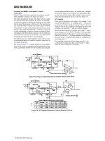
As NEMS and MEMS are used to control physical dynamic systems
(immune system or drug delivery, propeller or wing, relay or lock), to
illustrate the basic components, a high-level functional block diagram is
shown in Figure 2.1.4.
SensorActuator
−
SensorActuator
−
SensorActuator
−
Controller
rocessorP
Memories
IO
Antennas
ICs
NodeScalergeLa
−
NodeElementary
SensorActuator

−
SensorActuator
−
SensorActuator
−
SensorsActuators
nalTranslatioRotationa
−
/
Bus
© 2001 by CRC Press LLC
Figure 2.1.4. High-level functional block diagram of large-scale NEMS
and MEMS
For example, the desired flight path of aircraft (maneuvering and
landing) is maintained by displacing the control surfaces (ailerons and
elevators, canards and flaps, rudders and stabilizers) and/or changing the
control surface and wing geometry. Figure 2.1.5 documents the application
of the NEMS- and MEMS-based technology to actuate the control surfaces.
It should be emphasized that the NEMS and MEMS receive the digital
signal-level signals from the flight computer, and these digital signals are
converted into the desired voltages or currents fed to the microactuators or
electromagnetic flux intensity to displace the actuators. It is also important
that NEMS- and MEMS-based transducers can be used as sensors, and, as an
example, the loads on the aircraft structures during the flight can be
measured.
Data
Acquisition
Sensors




Antennas
Amplifiers
ICs
VariablesMeasured
Actuators
Analysisand
Decision
System
Dynamic
Controller
Output
VariablesSystem
Criteria
Objectives
VariablesMEMS
SensorActuator
−
MEMS
SensorActuator
−
SensorActuator
−
IO
© 2001 by CRC Press LLC
Figure 2.1.5. Aircraft with MEMS-based flight actuators
Microelectromechanical and Nanoelectromechanical Systems
Microelectromechanical systems are integrated microassembled
structures (electromechanical microsystems on a single chip) that have both
electrical-electronic (ICs) and mechanical components. To manufacture

MEMS, modified advanced microelectronics fabrication techniques and
materials are used. It was emphasized that sensing and actuation cannot be
viewed as the peripheral function in many applications. Integrated
actuators/sensors with ICs compose the major class of MEMS. Due to the use
of CMOS lithography-based technologies in fabrication actuators and
sensors, MEMS leverage microelectronics (signal processing, computing,
and control) in important additional areas that revolutionize the application
capabilities. In fact, MEMS have been considerably leveraged the
microelectronics industry beyond ICs. The needs to augmented actuators,
sensors, and ICs have been widely recognized. For example, mechatronics
concept, used for years in conventional electromechanical systems, integrates
all components and subsystems (electromechanical motion devices, power
converters, microcontrollers, et cetera). Simply scaling conventional
electromechanical motion devices and augmenting them with ICs have not
ψφθ
,,
:
AnglesEuler
ActuatorsFlight
BasedMEMS
−
SensorActuator −
SensorActuator
−
GeometryWing
GeometrySurface
ntDisplacemeSurface
Control
:
© 2001 by CRC Press LLC

met the needs, and theory and fabrication processes have been developed
beyond component replacement. Only recently it becomes possible to
manufacture MEMS at very low cost. However, there is a critical demand for
continuous fundamental, applied, and technological improvements, and
multidisciplinary activities are required. The general lack of synergy theory
to augment actuation, sensing, signal processing, and control is known, and
these issues must be addressed through focussed efforts. The set of long-
range goals has been emphasized in Chapter 1. The challenges facing the
development of MEMS are
•

advanced materials and process technology,
•

microsensors and microactuators, sensing and actuation mechanisms,
sensors-actuators-ICs integration and MEMS configurations,
•

packaging, microassembly, and testing,
•

MEMS modeling, analysis, optimization, and design,
•

MEMS applications and their deployment.
Significant progress in the application of CMOS technology enable the
industry to fabricate microscale actuators and sensors with the corresponding
ICs, and this guarantees the significant breakthrough. The field of MEMS has
been driven by the rapid global progress in ICs, VLSI, solid-state devices,
microprocessors, memories, and DSPs that have revolutionized

instrumentation and control. In addition, this progress has facilitated
explosive growth in data processing and communications in high-
performance systems. In microelectronics, many emerging problems deal
with nonelectric phenomena and processes (thermal and structural analysis
and optimization, packaging, et cetera). It has been emphasized that ICs is
the necessary component to perform control, data acquisition, and decision
making. For example, control signals (voltage or currents) are computer,
converted, modulated, and fed to actuators. It is evident that MEMS have
found application in a wide array of microscale devices (accelerometers,
pressure sensors, gyroscopes, et cetera) due to extremely-high level of
integration of electromechanical components with low cost and maintenance,
accuracy, reliability, and ruggedness. Microelectronics with integrated
sensors and actuators are batch-fabricated as integrated assemblies.
Therefore, MEMS can be defined as
batch-fabricated microscale devices (ICs and motion microstructures) that
convert physical parameters to electrical signals and vise versa, and in
addition, microscale features of mechanical and electrical components,
architectures, structures, and parameters are important elements of their
operation and design.
The manufacturability issues in NEMS and MEMS must be addressed. It
was shown that one can design and manufacture individually-fabricated
devices and subsystems. However, these devices and subsystems are unlikely
will be used due to very high cost.
© 2001 by CRC Press LLC
Piezoactuators and permanent-magnet technology has been used widely,
and rotating and linear electric transducers (actuators and sensors) are
designed. For example, piezoactive materials are used in ultrasonic motors.
Frequently, conventional concepts of the electric machinery theory
(rotational and linear direct-current, induction, and synchronous machine) are
used to design and analyze MEMS-based machines. The use of

piezoactuators is possible as a consequence of the discovery of advanced
materials in sheet and thin-film forms, especially PZT (lead zirconate
titanate) and polyvinylidene fluoride. The deposition of thin films allows
piezo-based electric machines to become a promising candidate for
microactuation in lithography-based fabrication. In particular, microelectric
machines can be fabricated using a deep x-ray lithography and
electrodeposition process. Two-pole synchronous and induction micro-
motors have been fabricated and tested.
To fabricate nanoscale structures, devices, and NEMS, molecular
manufacturing methods and technologies must be developed. Self- and
positional-assembly concepts are the preferable technologies compared
with individually-fabricated in the synthesis and manufacturing of
molecular structures. To perform self- and positional-assembly,
complementary pairs (CP) and molecular building blocks (MBB) should be
designed. These CP or MBB, which can be built from a couple to
thousands atoms, can be studied and designed using the DNA analogy. The
nucleic acids consist of two major classes of molecules (DNA and RNA).
Deoxyribonucleic acid (DNA) and ribonucleic acid (RNA) are the largest
and most complex organic molecules which are composed of carbon,
oxygen, hydrogen, nitrogen, and phosphorus. The structural units of DNA
and RNA are nucleotides, and each nucleotide consists of three
components (nitrogen-base, pentose and phosphate) joined by dehydration
synthesis. The double-helix molecular model of DNA was discovered by
Watson and Crick in 1953. The DNA (long double-stranded polymer with
double chain of nucleotides held together by hydrogen bonds between the
bases), as the genetic material (genes), performs two fundamental roles. It
replicates (identically reproduces) itself before a cell divides, and provides
pattern for protein synthesis directing the growth and development of all
living organisms according to the information DNA supports. The DNA
architecture provides the mechanism for the replication of genes. Specific

pairing of nitrogenous bases obey base-pairing rules and determine the
combinations of nitrogenous bases that form the rungs of the double helix.
In contrast, RNA carries (performs) the protein synthesis using the DNA
information. Four DNA bases are: A (adenine), G (guanine), C (cytosine),
and T (thymine). The ladder-like DNA molecule is formed due to
hydrogen bonds between the bases which paired in the interior of the
double helix (the base pairs are 0.34 nm apart and there are ten pairs per
turn of the helix). Two backbones (sugar and phosphate molecules) form
the uprights of the DNA molecule, while the joined bases form the rungs.
© 2001 by CRC Press LLC
Figure 2.1.6 illustrates that the hydrogen bonding of the bases are: A bonds
to T, G bonds to C. The complementary base sequence results.
Figure 2.1.6. DNA pairing due to hydrogen bonds
In RNA molecules (single strands of nucleotides), the complementary
bases are A bonds to U (uracil), and G bonds to C. The complementary base
bonding of DNA and RNA molecules gives one the idea of possible sticky-
ended assembling (through complementary pairing) of NEMS structures and
devices with the desired level of specificity, architecture, topology, and
organization. In structural assembling and design, the key element is the
ability of CP or MBB (atoms or molecules) to associate with each other
(recognize and identify other atoms or molecules by means of specific base
pairing relationships). It was emphasized that in DNA, A (adenine) bonds to
T (thymine) and G (guanine) bonds to C (cytosine). Using this idea, one can
design the CP such as A
1
-A
2
, B
1
-B

2
, C
1
-C
2
, etc. That is, A
1
pairs with A
2
,
while B
1
pairs with B
2
. This complementary pairing can be studied using
electromagnetics (Coulomb law) and chemistry (chemical bonding, for
example, hydrogen bonds in DNA between nitrogenous bases A and T, G
and C). Figure 2.1.7 shows how two nanoscale elements with sticky ends
form the complementary pair. In particular, "+" is the sticky end and "-" is its
complement. That is, the complementary pair A
1
-A
2
results.
Figure 2.1.7. Sticky ended electrostatically complementary pair A
1
-A
2
An example of assembling a ring is illustrated in Figure 2.1.8. Using the
sticky ended segmented (asymmetric) electrostatically CP, self-assembling of

TA
−
O
H
N-H O
N H-N
3
CH
Sugar
NN
CG
−
N-H O
H
O H-N
N-H N
Sugar
NN
N
N
Sugar
H
N
N
Sugar
−
2
q
+
1

q
1
A
2
A
1
A
2
A
+
1
q
−
2
q
© 2001 by CRC Press LLC
nanostructure is performed in the XY plane. It is evident that three-
dimensional structures can be formed through the self-assembling.
Figure 2.1.8. Ring self-assembling
It is evident that there are several advantages to use sticky ended
electrostatic CP. In the first place, the ability to recognize (identify) the
complementary pair is clear and reliably predicted. The second advantage is
the possibility to form stiff, strong, and robust structures.
Self-assembled complex nanostructures can be fabricated using
subsegment concept to form the branched junctions. This concept is well-
defined electrostatically and geometrically through Coulomb law and
branching connectivity. Using the subsegment concept, ideal objects (e.g.,
cubes, octahedron, spheres, cones, et cetera) can be manufactured.
Furthermore, the geometry of nanostructures can be easily controlled by the
number of CP and pairing MBB. It must be emphasized that it is possible to

generate a quadrilateral self-assembled nanostructure by using four and more
different CP. That is, in addition to electrostatic CP, chemical CP can be
used. Single- and double-stranded structures can be generated and linked in
the desired topological and architectural manners. The self-assembling must
be controlled during the manufacturing cycle, and CP and MBB, which can
be paired and topologically/architecturally bonded, must be added in the
desired sequence. For example, polyhedral and octahedral synthesis can be
performed when building elements (CP or MBB) are topologically or
geometrically specified. The connectivity of nanostructures determines the
minimum number of linkages that flank the branched junctions. The synthesis
of complex three-dimensional nanostructures is the design of topology, and
the structures are characterized by their branching and linking.
Linkage Groups in Molecular Building Blocks
The hydrogen bonds, which are weak, hold DNA and RNA strands.
Strong bonds are desirable to form stiff, strong, and robust nano- and
microstructures. Using polymer chemistry, functional groups which couple
−
2
q
+
1
q
+
1
q
© 2001 by CRC Press LLC
monomers can be designed. However, polymers made from monomers with
only two linkage groups do not exhibit the desired stiffness and strength.
Tetrahedral MBB structures with four linkage groups result in stiff and
robust structures. Polymers are made from monomers, and each monomer

reacts with two other monomers to form linear chains. Synthetic and organic
polymers (large molecules) are nylon and dacron (synthetic), and proteins
and RNA, respectively.
There are two major ways to assemble parts. In particular, self assembly
and positional assembly. Self-assembling is widely used at the molecular
scale, and the DNA and RNA examples were already emphasized. Positional
assembling is widely used in manufacturing and microelectronic
manufacturing. The current inability to implement positional assembly at the
molecular scale with the same flexibility and integrity that it applied in
microelectronic fabrication limits the range of nanostructures which can be
manufactured. Therefore, the efforts are focused on developments of MBB,
as applied to manufacture nanostructures, which guarantee:
•

mass-production at low cost and high yield;
•

simplicity and predictability of synthesis and manufacturing;
•

high-performance, repeatability, and similarity of characteristics;
•

stiffness, strength, and robustness;
•

tolerance to contaminants.
It is possible to select and synthesize MBB that satisfy the requirements
and specifications (non-flammability, non-toxicity, pressure, temperatures,
stiffness, strength, robustness, resistivity, permiability, permittivity, et

cetera). Molecular building blocks are characterized by the number of
linkage groups and bonds. The linkage groups and bonds that can be used to
connect MBB are:
•

dipolar bonds (weak),
•

hydrogen bonds (weak),
•

transition metal complexes bonds (weak),
•

amide and ester linkages (weak and strong).
It must be emphasized that large molecular building blocks (LMMB) can
be made from MBB. There is a need to synthesize robust three-dimensional
structures. Molecular building blocks can form planar structures with are
strong, stiff, and robust in-plane, but weak and compliant in the third
dimension. This problem can be resolved by forming tubular structures. It
was emphasized that it is difficult to form three-dimensional structures using
MBB with two linkage groups. Molecular building blocks with three linkage
groups form planar structures, which are strong, stiff, and robust in plane but
bend easily. This plane can be rolled into tubular structures to guarantee
stiffness. Molecular building blocks with four, five, six, and twelve linkage
groups form strong, stiff, and robust three-dimensional structures needed to
synthesize robust nano- and microstructures.
Molecular building blocks with L linkage groups are paired forming L-
pair structures, and planar and non-planar (three-dimensional) nano- and
© 2001 by CRC Press LLC

microstructures result. These MBB can have in-plane linkage groups and out-
of-plane linkage groups which are normal to the plane. For example,
hexagonal sheets are formed using three in-plane linkage groups (MBB is a
single carbon atom in a sheet of graphite) with adjacent sheets formed using
two out-of-plane linkage groups. It is evident that this structure has
hexagonal symmetry.
Molecular building blocks with six linkage groups can be connected
together in the cubic structure. These six linkage groups corresponding to six
sides of the cube or rhomb. Thus, MBB with six linkage groups form solid
three-dimensional structures as cubes or rhomboids. It should be emphasized
that buckyballs (C
60
), which can be used as MMB, are formed with six
functional groups. Molecular building blocks with six in-plane linkage
groups form strong planar structures. Robust, strong, and stiff cubic or
hexagonal closed-packed crystal structures are formed using twelve linkage
groups. Molecular building blocks synthesized and applied should guarantee
the desirable performance characteristics (stiffness, strength, robustness,
resistivity, permiability, permittivity, et cetera) as well as manufacturability.
It is evident that stiffness, strength, and robustness are predetermined by
bonds (weak and strong), while resistivity, permiability and permittivity are
the functions of MBB compounds and media.
© 2001 by CRC Press LLC
2.2. ELECTROMAGNETICS AND ITS APPLICATION FOR NANO-
AND MICROSCALE ELECTROMECHANICAL MOTION DEVICES
To study NEMS and MEMS actuators and sensors, smart structures, ICs
and antennas, one applies the electromagnetic field theory. Electric force holds
atoms and molecules together. Electromagnetics plays a central role in
molecular biology. For example, two DNA (deoxyribonucleic acid) chains
wrap about one another in the shape of a double helix. These two strands are

held together by electrostatic forces. Electric force is responsible for energy-
transforming processes in all living organisms (metabolism). Electromagnetism
is used to study protein synthesis and structure, nervous system, etc.
Electrostatic interaction was investigated by Charles Coulomb.
For charges q
1
and q
2
, separated by a distance x in free space, the
magnitude of the electric force is
F
q q
x
=
1 2
0
2
4πε
,
where
ε
0
is the permittivity of free space,
ε
0
= 8.85×10
−12
F/m or C
2
/N-m

2
,
1
4
9 10
0
9
πε
= ×
N-m
2
/C.
The unit for the force is the newton N, while the charges are given in
coulombs, C.
The force is the vector, and we have
r
r
F
q q
x
a
x
=
1 2
0
2
4πε
,
where
r

a
x
is the unit vector which is directed along the line joining these two
charges.
The capacity, elegance and uniformity of electromagnetics arise from a
sequence of fundamental laws linked one to other and needed to study the field
quantities.
Using the Gauss law and denoting the vector of electric flux density as
r
D
[F/m] and the vector of electric field intensity as
r
E
[V/m or N/C], the total
electric flux
Φ
[C] through a closed surface is found to be equal to the total
force charge enclosed by the surface. That is, one finds
Φ = ⋅ =
∫
r
r
D ds Q
s
s
,
r
r
D E= ε ,
where

ds
r
is the vector surface area, ds dsa
n
r
r
= ,
r
a
n
is the unit vector which is
normal to the surface;
ε
is the permittivity of the medium; Q
s
is the total
charge enclosed by the surface.
Ohm’s law relates the volume charge density
r
J
and electric field
intensity
r
E
; in particular,
© 2001 by CRC Press LLC
r
r
J E= σ ,
where

σ
is the conductivity [A/V-m], for copper σ = ×58 10
7
. , and for
aluminum
σ = ×35 10
7
. .
The current i is proportional to the potential difference, and the resistivity
ρ
of the conductor is the ratio between the electric field
r
E
and the current
density
r
J
. Thus,
ρ =
r
r
E
J
.
The resistance r of the conductor is related to the resistivity and
conductivity by the following formulas
r
l
A
=

ρ
and r
l
A
=
σ
,
where l is the length; A is the cross-sectional area.
It is important to emphasize that the parameters of NEMS and MEMS
vary. Let us illustrate this using the simplest nano-structure used in NEMS and
MEMS. In particular, the molecular wire. The resistances of the ware vary due
to heating. The resistivity depends on temperature T [
o
C], and
( ) ( )
[
]
ρ ρ α α
ρ ρ
( ) T T T T T= + − + − +
0 1 0 2 0
2
1 ,
where
α
ρ1
and α
ρ2
are the coefficients.
As an example, over the small temperature range (up to 160

o
C) for copper
(the wire is filled with copper) at T
0
= 20
o
C, we have
(
)
[
]
ρ( ) . .T T= × + −
−
17 10 1 00039 20
8
.
To study NEMS and MEMS, the basic principles of electromagnetic
theory should be briefly reviewed.
The total magnetic flux through the surface is given by
Φ = ⋅
∫
r
r
B ds ,
where
r
B
is the magnetic flux density.
The Ampere circuital law is
r

r
r
r
B dl J ds
l s
⋅ = ⋅
∫ ∫
µ
0
,
where
µ
o
is the permeability of free space,
µ
o
= 4π×10
−7
H/m or T-m/A.
For the filamentary current, Ampere’s law connects the magnetic flux with
the algebraic sum of the enclosed (linked) currents (net current) i
n
, and
r
r
B dl i
l
o n
⋅ =
∫

µ .
The time-varying magnetic field produces the electromotive force (emf),
denoted as , which induces the current in the closed circuit. Faraday’s law
© 2001 by CRC Press LLC
relates the emf, which is merely the induced voltage due to conductor motion in
the magnetic field, to the rate of change of the magnetic flux
Φ
penetrating in
the loop. In approaching the analysis of electromechanical energy
transformation in NEMS and MEMS, Lenz’s law should be used to find the
direction of emf and the current induced. In particular, the emf is in such a
direction as to produce a current whose flux, if added to the original flux, would
reduce the magnitude of the emf. According to Faraday’s law, the induced emf
in a closed-loop circuit is defined in terms of the rate of change of the magnetic
flux
Φ
as

= ⋅ = − ⋅ = − = −
∫ ∫
r
r
r
r
E t dl
d
dt
B t ds N
d
dt

d
dt
l s
( ) ( )
Φ ψ
,
where N is the number of turns;
ψ
denotes the flux linkages.
This formula represents the Faraday law of induction, and the induced emf
(induced voltage), as given by

= − = −
d
dt
N
d
dt
ψ Φ
,
is a particular interest
The current flows in an opposite direction to the flux linkages. The
electromotive force (energy-per-unit-charge quantity) represents a magnitude
of the potential difference V in a circuit carrying a current. One obtains,
V = − ir +
= − −ir
d
dt
ψ
.

The unit for the emf is volts.
The Kirchhoff voltage law states that around a closed path in an electric
circuit, the algebraic sum of the emf is equal to the algebraic sum of the voltage
drop across the resistance.
Another formulation is: the algebraic sum of the voltages around any
closed path in a circuit is zero.
The Kirchhoff current law states that the algebraic sum of the currents at
any node in a circuit is zero.
The magnetomotive force (mmf) is the line integral of the time-varying
magnetic field intensity
r
H t( ) ; that is,
mmf H t dl
l
= ⋅
∫
r
r
( ) .
One concludes that the induced mmf is the sum of the induced current and
the rate of change of the flux penetrating the surface bounded by the contour.
To show that, we apply Stoke’s theorem to find the integral form of Ampere’s
law (second Maxwell’s equation), as given by
∫∫∫
+⋅=⋅
ssl
sd
dt
tDd
sdtJldtH

r
r
r
r
r
r
)(
)()(
,
where
r
J t( )
is the time-varying current density vector.
© 2001 by CRC Press LLC
The unit for the magnetomotive force is amperes or ampere-turns
The duality of the emf and mmf can be observed using
.
= ⋅
∫
r
r
E t dl
l
( ) and mmf H t dl
l
= ⋅
∫
r
r
( ) .

The inductance (the ratio of the total flux linkages to the current which
they link,
L
N
i
=
Φ
) and reluctance (the ratio of the mmf to the total flux,
ℜ =
mmf
Φ
) are used to find emf and mmf.
Using the following equation for the self-inductance
L
i
=
ψ
, we have

= − = − = − −
d
dt
d Li
dt
L
di
dt
i
dL
dt

ψ ( )
.
If L = const, one obtains

= −L
di
dt
.
That is, the self-inductance is the magnitude of the self-induced emf per
unit rate of change of current.
Example 2.2.1.
Find the self-inductances of a nano-solenoid with air-core and filled-core
(
o
µµ 100=
). The solenoid has 100 turns (N = 100), the length is 20 nm (l=20
nm), and the uniform circular cross-sectional area is
18
105
−
× m
2
(
18
105
−
×=A m
2
).
Solution. The magnetic field inside a solenoid is given by

B
Ni
l
=
µ
0
.
By using
= − = −N
d
dt
L
di
dt
Φ
and applying Φ = =BA
NiA
l
µ
0
,
one obtains
L
N A
l
=
µ
0
2
.

Then, L = 3.14×10
−12
H.
If solenoid is filled with a magnetic material, we have
L
N A
l
=
µ
2
, and L = 3.14×10
−9
H.
Example 2.2.2.
Derive a formula for the self-inductance of a torroidal solenoid which has a
rectangular cross section (2a × b) and mean radius r.
© 2001 by CRC Press LLC
Solution. The magnetic flux through a cross section is found as
Φ = = = =
+
−






−
+
−

+
−
+
∫ ∫ ∫
Bbdr
Ni
r
bdr
Nib
r
dr
Nib r a
r a
r a
r a
r a
r a
r a
r a
µ
π
µ
π
µ
π2 2
1
2
ln .

Hence,

L
N
i
N b r a
r a
= =
+
−






Φ µ
π
2
2
ln .
By studying the electromagnetic torque
r
T
[N-m] in a current loop, one
obtains the following equation
r
r
r
T
M
B

=
×
,
where
r
M
denotes the magnetic moment.
Let us examine the torque-energy relations in nano- and microscale
actuators. Our goal is to study the magnetic field energy. It is known that the
energy stored in the capacitor is
1
2
2
CV , while energy stored in the inductor is
1
2
2
Li . Observe that the energy in the capacitor is stored in the electric field
between plates, while the energy in the inductor is stored in the magnetic field
within the coils.
Let us find the expressions for energies stored in electrostatic and magnetic
fields in terms of field quantities. The total potential energy stored in the
electrostatic field is found using the potential difference V, and we have
W Vdv
e v
v
=
∫
1
2

ρ [J],
where
ρ
v
is the volume charge density [C/m
3
], ρ
v
D= ∇⋅
r
r
,
r
∇ is the curl
operator.
This expression for
W
e
is interpreted in the following way. The potential
energy should be found using the amount of work which is required to
position the charge in the electrostatic field. In particular, the work is found
as the product of the charge and the potential. Considering the region with a
continuous charge distribution (
ρ
v
const= ), each charge is replaced by
ρ
v
dv , and hence the equation W Vdv
e v

v
=
∫
1
2
ρ
results.
In the Gauss form, using
ρ
v
D= ∇⋅
r
r
and making use
r
r
E V= −∇ , one
obtains the following expression for the energy stored in the electrostatic
field
W D Edv
e
v
= ⋅
∫
1
2
r
r
,
and the electrostatic volume energy density is

1
2
r
r
D E⋅ [J/m
3
].
© 2001 by CRC Press LLC
For a linear isotropic medium W E dv D dv
e
v v
= =
∫ ∫
1
2
2
1
2
2
1
ε
ε
r
r
.
The electric field
r
E x y z( , , ) is found using the scalar electrostatic
potential function
V x y z( , , ) as

r
r
E x y z V x y z( , , ) ( , , )= −∇ .
In the cylindrical and spherical coordinate systems, we have
r
r
E r z V r z( , , ) ( , , )φ φ= −∇ and
r
r
E r V r( , , ) ( , , )θ φ θ φ= −∇ .
Using
W Vdv
e v
v
=
∫
1
2
ρ , the potential energy which is stored in the
electric field between two surfaces (for example, in capacitor) is found to be
W QV CV
e
= =
1
2
1
2
2
.
Using the principle of virtual work, for the lossless conservative system,

the differential change of the electrostatic energy
dW
e
is equal to the
differential change of mechanical energy
dW
mec
; that is
dW dW
e mec
=
.
For translational motion
dW F dl
mec e
= ⋅
r
r
,
where
dl
r
is the differential displacement.
One obtains
dW W dl
e e
= ∇ ⋅
r
r
.

Hence, the force is the gradient of the stored electrostatic energy,
r
r
F W
e e
= ∇ .
In the Cartesian coordinates, we have
F
W
x
F
W
y
ex
e
ey
e
= =
∂
∂
∂
∂
,
and F
W
z
ez
e
=
∂

∂
.
Example 2.2.3.
Consider the capacitor (the plates have area A and they are separated by x),
which is charged to a voltage V. The permittivity of the dielectric is
ε
. Find the
stored electrostatic energy and the force
F
ex
in the x direction.
Solution. Neglecting the fringing effect at the edges, one concludes that
the electric field is uniform, and
E
V
x
= . Therefore, we have

W E dv
V
x
dv
V
x
Ax
A
x
V C x V
e
v v

= =






= = =
∫ ∫
1
2
2
1
2
2
1
2
2
2
1
2
2
1
2
2
ε ε ε ε
r
( ) .
Thus, the force is
© 2001 by CRC Press LLC

(
)
F
W
x
C x V
x
V
C x
x
ex
e
= = =
∂
∂
∂
∂
∂
∂
1
2
2
1
2
2
( )
( )
To find the stored energy in the magnetostatic field in terms of field
quantities, the following formula is used
W B Hdv

m
v
= ⋅
∫
1
2
r
r
.
The magnetic volume energy density is
1
2
r
r
B H
⋅
[J/m
3
].
Using
r
r
B H= µ , one obtains two alternative formulas
W H dv
B
dv
m
v v
= =
∫ ∫

1
2
2
1
2
2
µ
µ
r
r
.
To show how the energy concept studied is applied to electromechanical
devices, we find the energy stored in inductors. To approach this problem,
we substitute
r
r
r
B A= ∇ × , and using the following vector identity
(
)
r
r
r
r
r
r
r
r
r
H A A H A H

⋅∇ × = ∇⋅ × + ⋅∇ ×
, one obtains

(
)
( )
.
2
1
2
1
2
1
2
1
2
1
2
1
∫∫∫
∫∫∫
⋅=⋅+⋅×=
×∇⋅+×⋅∇=⋅=
vvs
vvv
m
dvJAdvJAsdHA
dvHAdvHAdvHBW
r
r

r
r
r
r
r
r
r
r
r
r
r
r
r
Using the general expression for the vector magnetic potential
(
)
r
r
A r
[Wb/m], as given by
( )
(
)
r
r
r
r
A r
J r
x

dv
A
J
v
A
=
∫
µ
π
0
4
,
r
r
∇⋅ =A 0,
we have
(
)
(
)
W
J r J r
x
dv dv
m
A
J
vv
J
=

⋅
∫∫
µ
π8
r
r
r
r
.
Here,
v
J
is the volume of the medium where
r
J
exists.
The general formula for the self-inductance
i
j
=
and the mutual
inductance
i
j
≠
of loops i and j is
L
N
i i
ij

i ij
j
ij
j
= =
Φ
ψ
,
where
ψ
ij
is the flux linkage through ith coil due to the current in jth coil; i
j
is
the current in jth coil.
© 2001 by CRC Press LLC
The Neumann formula is applied to find the mutual inductance. We have,
L L
dl dl
x
i j
ij ji
j i
ij
ll
ji
= =
⋅
≠
∫∫

µ
π4
r
r
, .
Then, using
(
)
(
)
W
J r J r
x
dv dv
m
A
J
vv
J
=
⋅
∫∫
µ
π8
r
r
r
r
, one obtains
W

i dl i dl
x
m
j j i i
ij
ll
ji
=
⋅
∫∫
µ
π8
r
r
.
Hence, the energy stored in the magnetic field is found to be
W i L i
m i ij j
=
1
2
.
As an example, the energy, stored in the inductor is
W Li
m
=
1
2
2
.

The differential change in the stored magnetic energy should be found.
Using
dW
dt
L i
di
dt
L i
di
dt
i i
dL
dt
m
ij j
i
ij i
j
i j
ij
= + +











1
2
,
we have
dW L i di L i di i i dL
m ij j i ij i j i j ij
= + +






1
2
.
For translational motion, the differential change in the mechanical energy
is expressed by
dW F dl
mec m
= ⋅
r
r
.
Assuming that the system is conservative (for lossless systems
dW dW
mec m
=
), in the rectangular coordinate system we obtain the following

equation
dW
W
x
dx
W
y
dy
W
z
dz W dl
m
m m m
m
= + + = ∇ ⋅
∂
∂
∂
∂
∂
∂
r
r
.
Hence, the force is the gradient of the stored magnetic energy, and
r
r
F W
m m
= ∇ .

In the XYZ coordinate system for the translational motion, we have
F
W
x
F
W
y
mx
m
my
m
= =
∂
∂
∂
∂
,
and F
W
z
mz
m
=
∂
∂
.
For the rotational motion, the torque should be used. Using the differential
change in the mechanical energy as a function of the angular displacement
θ
,

the following formula results if the rigid body (nano- or microactuator) is
constrained to rotate about the z-axis
dW T d
mec e
= θ
,
where
T
e
is the z-component of the electromagnetic torque.
© 2001 by CRC Press LLC
Assuming that the system is lossless, one obtains the following expression
for the electromagnetic torque
T
W
e
m
=
∂
∂θ
.
Example 2.2.4.
Calculate the magnetic energy of the torroidal microsolenoid if the
self-inductance is 1×10
−10
H (L=2×10
−10
H) when the current is 0.001 A
(i=0.001 A).
Solution. The stored field energy is

W Li
m
=
1
2
2
,
therefore
1310
2
1
101001.0102
−−
×=××=
m
W J.
Example 2.2.5.
Calculate the force developed by the microelectromagnet with the cross-
sectional area A if the current i
a
(t) in and N coils produces the constant flux
m
Φ
, see Figure 2.2.1.
)(tx
)(ti
Magnetic force F
mx
,
Φ

m
N
Spring k
s
,
Figure 2.2.1. Microelectromagnet
Solution.
From
W H dv
B
dv
m
v v
= =
∫ ∫
1
2
2
1
2
2
µ
µ
r
r
, for the virtual displacement dy,
assuming that the flux is constant and taking into the account the fact that the
displacement changes only the magnetic energy stored in the air gaps, we
have
© 2001 by CRC Press LLC

dy
A
Ady
B
dWdW
m
gapairmm
0
2
0
2
2
2
µµ
Φ
===
.
Thus, if
m
Φ
=const, one concludes that the increase of the air gap (dy)
leads to increase of the stored magnetic energy, and from
x
W
F
m
mx
∂
∂
= one

finds the expression for the force
A
aF
m
ymx
0
2
µ
Φ
−=
r
r
.
The result indicates that the force tends to reduce the air-gap length, and
the movable member is attached to the spring which develops the force which
opposite to the electromagnetic force.
In nano- and microscale electromechanical motion devices, the coupling
(magnetic interaction) between windings that are carrying currents is
represented by their mutual inductances. In fact, the current in each winding
causes the magnetic field in other windings. The mutually induced emf is
characterized by the mutual inductance which is a function of the position x or
the angular displacement
θ
. By applying the expression for the coenergy
[
]
W i L x
c
, ( ) or
(

)
[
]
W i L
c
, θ , the developed electromagnetic torque can be
easily found. In particular,
T i x
W i L x
x
e
c
( , )
[ , ( )]
=
∂
∂
and T i x
W i L
e
c
( , )
[ , ( )]
=
∂ θ
∂θ
.
Example 2.2.6.
Consider the microelectromagnet which has N turns, see Figure 2.2.2.
The distance between the stationary and movable members is denoted as

x t( ) . The mean lengths of the stationary and movable members are l
1
and
l
2
, and the cross-sectional area is A. Neglecting the leakage flux, find the
force exerted on the movable member if the time-varying current
i t
a
( ) is
supplied. The permeabilities of stationary and movable members are
µ
1
and
µ
2
.
© 2001 by CRC Press LLC
x t( )
i t
a
( )
Spring k
s
,
Magnetic force F
mx
,
Φ
m

l
2
l
1
N
µ
1
µ
2
Figure 2.2.2. Schematic of an electromagnet
Solution.
The magnetostatic force is
F
W
x
mx
m
=
∂
∂
,
where
W Li t
m a
=
1
2
2
( ) .
The magnetizing inductance should be calculated, and we have

L
N
i t i t
a a
= =
Φ
( ) ( )
ψ
,
where the magnetic flux is
Φ =
ℜ + ℜ + ℜ + ℜ
Ni t
a
x x
( )
1 2
.
The reluctances of the ferromagnetic materials of stationary and movable
members
ℜ
1
and ℜ
2
, as well as the reluctance of the air gap ℜ
x
, are
found as
ℜ =
1

1
0 1
l
Aµ µ
,
ℜ =
2
2
0 2
l
Aµ µ
and
ℜ =
x
x t
A
( )
µ
0
and the circuit analog with the reluctances of the various paths is illustrated
in Figure 2.2.3.
© 2001 by CRC Press LLC
Ni t
a
( )
ℜ
1
ℜ
x
ℜ

2
ℜ
x
Figure 2.2.3. Circuit analog
By making use the reluctances in the movable and stationary members
and air gap, one obtains the following formula for the flux linkages
ψ
µ µ µ µ µ
= =
+ +
N
N i t
l
A
x t
A
l
A
a
Φ
2
1
0 1 0
2
0 2
2
( )
( )
,
and the magnetizing inductance is a nonlinear function of the displacement. We

have
L x
N
l
A
x t
A
l
A
N A
l x t l
( )
( )
( )
=
+ +
=
+ +
2
1
0 1 0
2
0 2
2
0 1 2
2 1 1 2 1 2
2
2
µ µ µ µ µ
µ µ µ

µ µ µ µ
.
Using
(
)
(
)
F
W
x
L x t i t
x
mx
m
a
= =
∂
∂
∂
∂
1
2
2
( ) ( )
, the force in the x direction is
found to be
F
N Ai
l x t l
mx

a
= −
+ +
2
0 1
2
2
2 2
2 1 1 2 1 2
2
µ µ µ
µ µ µ µ( )
.
It should be emphasized that as differential equations must be developed
to model the microelectromagnet studied. Using Newton’s second law of
motion, one obtains
dx
dt
v= ,
dv
dt m
N Ai
l x t l
k x
a
s
= −
+ +
−







1
2
2
0 1
2
2
2 2
2 1 1 2 1 2
2
µ µ µ
µ µ µ µ( )
.
Example 2.2.7.
Two micro-coils have mutual inductance 0.00005 H (L
12
=0.00005 H). The
current in the first coil is
i t
1
4
=
sin
. Find the induced emf in the second
coil.
© 2001 by CRC Press LLC

Solution.
The induced emf is given as
2
= L
di
dt
12
1
.
By using the power rule for the time-varying current in the first coil
i t
1
4= sin , we have
di
dt
t
t
1
2 4
4
=
cos
sin
.
Hence,
2

t
t
4sin

4cos0001.0
=
.
Basic Foundations in Model Developments of Nano- and
Microactuators in Electromagnetic Fields
Electromagnetic theory and mechanics form the basis for the
development of NEMS and MEMS models.
The electrostatic and magnetostatic equations in linear isotropic media
are found using the vectors of the electric field intensity
E
r
, electric flux
density
D
r
, magnetic field intensity
H
r
, and magnetic flux density
B
r
. In
addition, one uses the constitutive equations
ED
r
r
ε= and HB
r
r
µ=

where
ε
is the permittivity;
µ
is the permiability.
The basic equations are given in the Table 1.
Table 2.2.1.
Fundamental Equations of Electrostatic and Magnetostatic Fields
Electrostatic Model Magnetostatic Model
Governing
equations
0),,,( =×∇ tzyxE
r
ε
ρ
),,,(
),,,(
tzyx
tzyxE
v
=⋅∇
r
0),,,( =×∇ tzyxH
r
0),,,( =⋅∇ tzyxH
r
Constitutive
equations
ED
r

r
ε= HB
r
r
µ=
In the static (time-invariant) fields, electric and magnetic field vectors
form separate and independent pairs. That is,
E
r
and
D
r
are not related to
H
r
and
B
r
, and vice versa. However, in reality, the electric and magnetic fields are
time-varying, and the changes of magnetic field influence the electric field, and
vice versa.
© 2001 by CRC Press LLC