Tài liệu Image and Videl Comoression P13 doc

14

© 2000 by CRC Press LLC

Further Discussion
and Summary on
2-D Motion Estimation

Since Chapter 10, we have been devoting our discussion to motion analysis and motion-compen-
sated coding. Following a general description in Chapter 10, three major techniques — block
matching, pel recursion, and optical flow — are covered in Chapters 11, 12, and 13, respectively.
In this chapter, before concluding this subject, we provide further discussion and a summary.
A general characterization for 2-D motion estimation, thus for all three techniques, is given in
Section 14.1. In Section 14.2, different classifications of various methods for 2-D motion analysis
are given in a wider scope. Section 14.3 is concerned with a performance comparison among the
three major techniques. More-advanced techniques and new trends in motion analysis and motion
compensation are introduced in Section 14.4.

14.1 GENERAL CHARACTERIZATION

A few common features characterizing all three major techniques are discussed in this section.

14.1.1 A

PERTURE

P

ROBLEM

The aperture problem, discussed in Chapter 13, describes phenomena that occur when observing
motion through a small opening in a flat screen. That is, one can only observe normal velocity. It
is essentially a form of ill-posed problem since it is concerned with existence and uniqueness issues,
as illustrated in Figure 13.2(a) and (b). This problem is inherent with the optical flow technique.
We note, however, that the aperture problem also exists in block matching and pel recursive
techniques. Consider an area in an image plane having strong intensity gradients. According to our
discussion in Chapter 13, the aperture problem does exist in this area no matter what type of
technique is applied to determine local motion. That is, motion perpendicular to the gradient cannot
be determined as long as only a local measure is utilized. It is noted that, in fact, the steepest
descent method of the pel recursive technique only updates the estimate along the gradient direction
(Tekalp, 1995).

14.1.2 I

LL

-P

OSED

I

NVERSE

P

ROBLEM

In Chapter 13, when we discuss the optical flow technique, a few fundamental issues are raised. It
is stated that optical flow computation from image sequences is an inverse problem, which is usually

ill-posed. Specifically, there are three problems: nonexistence, nonuniqueness, and instability. That
is, the solution may not exist; if it exists, it may not be unique. The solution may not be stable in
the sense that a small perturbation in the image data may cause a huge error in the solution.
Now we can extend our discussion to both block matching and pel recursion. This is because
both block matching and pel recursive techniques are intended for determining 2-D motion from
image sequences, and are therefore inverse problems.

© 2000 by CRC Press LLC

14.1.3 C

ONSERVATION

I

NFORMATION



AND

N

EIGHBORHOOD

I

NFORMATION

Because of the ill-posed nature of 2-D motion estimation, a unified point of view regarding various

optical flow algorithms is also applicable for block matching and pel recursive techniques. That is,
all three major techniques involve extracting conservation information and extracting neighborhood
information.
Take a look at the block-matching technique. There, conservation information is a distribution
of some sort of features (usually intensity or functions of intensity) within blocks. Neighborhood
information manifests itself in that all pixels within a block share the same displacement. If the
latter constraint is not imposed, block matching cannot work. One example is the following extreme
case. Consider a block size of 1

¥

1, i.e., a block containing only a single pixel. It is well known
that there is no way to estimate the motion of a pixel whose movement is independent of all its
neighbors (Horn and Schunck, 1981).
With the pel recursive technique, say, the steepest descent method, conservation information
is the intensity of the pixel for which the displacement vector is to be estimated. Neighborhood
information manifests itself as recursively propagating displacement estimates to neighboring pixels
(spatially or temporally) as initial estimates.
In Section 12.3, it is pointed out that Netravali and Robbins suggested an alternative, called
“inclusion of a neighborhood area.” That is, in order to make displacement estimation more robust,
they consider a small neighborhood

W

of the pixel for evaluating the square of displaced frame
difference (DFD) in calculating the update term. They assume a constant displacement vector within
the area. The algorithm thus becomes
(14.1)
where

i

represents an index for the

i

th pixel (

x

,

y

) within

W

, and

w

i

is the weight for the

i

th pixel
in

W

. All the weights satisfy certain conditions; i.e., they are nonnegative, and their sum equals 1.
Obviously, in this more-advanced algorithm, the conservation information is the intensity distribu-
tion within the neighborhood of the pixel, the neighborhood information is imposed more explicitly,
and it is stronger than that in the steepest descent method.

14.1.4 O

CCLUSION



AND

D

ISOCCLUSION

The problems of occlusion and disocclusion make motion estimation more difficult and hence more
challenging. Here we give a brief description about these and other related concepts.
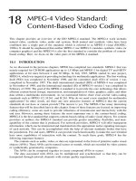
Let us consider Figure 14.1. There, the rectangle

ABCD

represents an object in an image taken
at the moment of

t

n

-1

,

f

(

x

,

y

,

t

n

-1

). The rectangle EFGH denotes the same object, which has been
translated, in the image taken at

t

n

moment,

f

(

x

,

y

,

t

n

). In the image

f

(

x

,

y

,

t

n

), the area

BFDH

is
occluded by the object that newly moves in. On the other hand, in

f

(

x

,

y

,

t

n

), the area of

AECG

resurfaces and is referred to as a newly visible area, or a newly exposed area.
Clearly, when occlusion and disocclusion occur, all three major techniques discussed in this
part will encounter a fatal problem, since conservation information may be lost, making motion
estimation fail in the newly exposed areas. If image frames are taken densely enough along the
temporal dimension, however, occlusion and disocclusion may not cause serious problems, since
the failure in motion estimation may be restricted to some limited areas. An extra bit rate paid for
the corresponding increase in encoding prediction error is another way to resolve the problem. If
high quality and low bit rate are both desired, then some special measures have to be taken.
One of the techniques suitable for handling the situation is Kalman filtering, which is known
as the best, by almost any reasonable criterion, technique working in the Gaussian white noise case
vv v
v
d d w DFD x y d
kk
d
i
k
ixy Q
+
Œ
=-—
()
Â
12
1

2
a ,,; ,
,,

© 2000 by CRC Press LLC

(Brown and Hwang, 1992). If we consider the system that estimates the 2-D motion to be contam-
inated by Gaussian white noise, we can use Kalman filtering to increase the accuracy of motion
estimation, particularly along motion discontinuities. It is powerful in doing incremental, dynamic,
and real-time estimation.
In estimating 3-D motion, Kalman filtering was applied by Matthies et al. (1989) and Pan et al.
(1994). Kalman filters were also utilized in optical flow computation (Singh, 1992; Pan and Shi,
1994). In using the Kalman filter technique, the question of how to handle the newly exposed areas
was raised by Matthies et al. (1989). Pan et al. (1994) proposed one way to handle this issue, and
some experimental work demonstrated its effectiveness.

14.1.5 R

IGID



AND

N

ONRIGID

M

OTION

There are two types of motion: rigid motion and nonrigid motion. Rigid motion refers to motion
of rigid objects. It is known that our human vision system is capable of perceiving 2-D projections
of 3-D moving rigid bodies as 2-D moving rigid bodies. Most cases in computer vision are concerned
with rigid motion. Perhaps this is due to the fact that most applications in computer vision fall into
this category. On the other hand, rigid motion is easier to handle than nonrigid motion. This can
be seen in the following discussion.
Consider a point

P

in 3-D world space with the coordinates (

X

,

Y

,

Z

), which can be represented
by a column vector :
(14.2)
Rigid motion involves rotation and translation, and has six free motion parameters. Let

R

denote
the rotation matrix and

T

the translational vector. The coordinates of point

P

in the 3-D world after
the rigid motion are denoted by

¢

. Then we have
(14.3)
Nonrigid motion is more complicated. It involves deformation in addition to rotation and translation,
and thus cannot be characterized by the above equation. According to the Helmholtz theory
(Sommerfeld, 1950), the counterpart of the above equation becomes
(14.4)
where

D

is a deformation matrix. Note that

R

,

T

, and

D

are pixel dependent. Handling nonrigid
motion, hence, is very complicated.

FIGURE 14.1

Occlusion and disocclusion.
v
v
v
vXYZ
T
=
()
,, .
v
v
vv
¢
=+vRvT.
vv v
¢
=++vRvTDv,

© 2000 by CRC Press LLC

In videophony and videoconferencing applications, a typical scene might be a head-and-
shoulder view of a person imposed on a background. The facial expression is nonrigid in nature.
Model-based facial coding has been studied extensively (Aizawa and Harashima, 1994; Li et al.,
1993; Arizawa and Huang, 1995). There, a 3-D wireframe model is used for handling rigid head
motion. Li (1993) analyzes the facial nonrigid motion as a weighted linear combination of a set of

action units

, instead of determining

D

directly. Since the number of action units is limited, the
compuatation becomes less expensive. In the Aizawa and Harashima (1989) paper, the portions in
the human face with rich expression, such as lips, are

cut

and then transmitted out. At the receiving
end, the portions are

pasted

back in the face.
Among the three types of techniques, block matching may be used to manage rigid motion,
while pel recursive and optical flow may be used to handle either rigid or nonrigid motion.

14.2 DIFFERENT CLASSIFICATIONS

There are various methods in motion estimation, which can be classified in many different ways.
We discuss some of the classifications in this section.

14.2.1 D

ETERMINISTIC

M

ETHODS



VS

. S

TOCHASTIC

M

ETHODS

Most algorithms are deterministic in nature. To see this, let us take a look at the most prominent
algorithm for each of the three major 2-D motion estimation techniques. That is, the Jain and Jain
algorithm for the block matching technique (Jain and Jain, 1981); the Netravali and Robbins
algorithm for the pel recursive technique (Netravali and Robbins, 1979); and the Horn and Schunck
algorithm for the optical flow technique (Horn and Schunck, 1981). All are deterministic methods.
There are also stochastic methods in 2-D motion estimation, such as the Konrad and Dubois

algorithm (Konrad and Dubois, 1992), which estimates 2-D motion using the maximum

a posteriori

probability (MAP).

14.2.2 S

PATIAL

D

OMAIN

M

ETHODS



VS

. F

REQUENCY

D

OMAIN

M

ETHODS

While most techniques in 2-D motion analysis are spatial domain methods, there are also frequency
domain methods (Kughlin and Hines, 1975; Heeger, 1988; Porat and Friedlander, 1990; Girod,
1993; Kojima et al., 1993; Koc and Liu, 1998). Heeger (1988) developed a method to determine
optical flow in the frequency domain, which is based on spatiotemporal filters. The basic idea and
principle of the method is introduced in this subsection. A very new and effective frequency method
for 2-D motion analysis (Koc and Liu, 1998) is presented in Section 14.4, where we discuss new
trends in 2-D motion estimation.

14.2.2.1 Optical Flow Determination Using Gabor Energy Filters

The frequency domain method of optical flow computation developed by Heeger is suitable for
highly textured image sequences. First, let us take a look at how motion can be detected in the
frequency domain.

Motion in the spatiotemporal frequency domain

— We initiate our discussion with a 1-D case.
The spatial frequency of a (translationally) moving sinusoidal signal,

w

x

, is defined as cycles per
distance (usually cycles per pixel), while temporal frequency,

w

t

, is defined as cycles per time unit
(usually cycles per frame). Hence, the velocity of (translational) motion, defined as distance per
time unit (usually pixels per frame), can be related to the spatial and temporal frequencies as follows.
(14.5)
v
v
v
tx
=w w .

© 2000 by CRC Press LLC

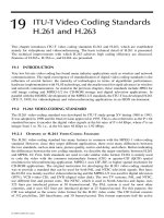
A 1-D moving signal with a velocity

v

may have multiple spatial frequency components. Each
spatial frequency component

w

xi

,

i

= 1,2,… has a corresponding temporal frequency component

w

ti

such that
(14.6)
This relation is shown in Figure 14.2. Thus, we see that in the spatiotemporal frequency domain,
velocity is the slope of a straight line relating temporal and spatial frequencies.
For 2-D moving signals, we denote spatial frequencies by

w

x

and

w

y

, and velocity vector by
= (

v

x

,

v

y

)

. The above 1-D result can be extended in a straightforward manner as follows:
(14.7)
The interpretation of Equation 14.7 is that a 2-D translating texture pattern occupies a plane in the
spatiotemporal frequency domain.

Gabor Energy Filters

— As Adelson and Bergen (1985) pointed out, the translational motion of
image patterns is characterized by orientation in the spatiotemporal domain. This can be seen from
Figure 14.3. Therefore, motion can be detected by using spatiotemporally oriented filters. One filter
of this type, suggested by Heeger, is the Gabor filter.
A 1-D sine-phase Gabor filter is defined as follows:
(14.8)
Obviously, this is a product of a sine function and a Gaussian probability density function. In the
frequency domain, this is the convolution between a pair of impulses located in

w

and –

w

, and the
Fourier transform of the Gaussian, which is itself again a Gaussian function. Hence, the Gabor
function is localized in a pair of Gaussian windows in the frequency domain. This means that the
Gabor filter is able to pick up some frequency components selectively.
A 3-D sine Gabor function is
(14.9)

FIGURE 14.2

Velocity in 1-D spatiotemporal frequency domain.
ww
ti xi
v= .
v
v
www
txxyy
vv=+.
gt t
t
()
=
p
p
()
-
Ï
Ì
Ó
¸

˝
˛
1
2
2
2
2
2
s
w
s
sin exp .
gxyt
xyt
xyt
xyt x y t
xyt
, , exp
sin ,
()
=
p
◊- ++
Ê
Ë
Á
ˆ
¯
˜
Ï

Ì
Ô
Ó
Ô
¸
˝
Ô
˛
Ô
◊p ++
()
[]
1
2
1
2
2
32
2
2
2
2
2
2
000
sss s s s
www

© 2000 by CRC Press LLC

where

s

x

,

s

y

, and

s

t

are, respectively, the spreads of the Gaussian window along the spatiotemporal
dimensions; and

w

x

0

,

w

y

0

, and

w

t

0

are, respectively, the central spatiotemporal frequencies. The
actual Gabor energy filter used by Heeger is the sum of a sine-phase filter (which is defined above),
and a cosine-phase filter (which shares the same spreads and central frequencies as that in the sine-
phase filter, and replaces sine by cosine in Equation 14.9). Its frequency response, therefore, is as
follows.
(14.10)
This indicates that the Gabor filter is motion sensitive in that it responds largely to motion that has
more power distributed near the central frequencies in the spatiotemporal frequency domain, while
it responds poorly to motion that has little power near the central frequencies.

Flow extraction with motion energy

— Using a vivid example, Heeger explains in his paper why
one such filter is not sufficient in detection of motion. Multiple Gabor filters must be used. In fact,
a set of 12 Gabor filters are utilized in Heeger’s algorithm. The 12 Gabor filters in the set have
one thing in common:
(14.11)

FIGURE 14.3

Orientation in spatiotemporal domain. (a) A horizontal bar translating downward. (b) A
spatiotemporal cube. (c) A slice of the cube perpendicular to

y

axis. The orientation of the slant edges represents
the motion.
G
xyt xx x yy y t t t
xx x yy y t t t
www sw w sw w sw w
sw w sw w sw w
, , exp
exp
()
=-p -
()
+-
()
+-
()
È
Î
Í
˘
˚
˙

Ï
Ì
Ó
¸
˝
˛
+-p +
()
++
()
++
()
È
1
4
4
1
4
4
22
2
2
2
2
2
22
2
2
2
2

2
000
000
ÎÎ
Í
˘
˚
˙
Ï
Ì
Ó
¸
˝
˛
.
www
00
2
0
2
=+
xy
.
© 2000 by CRC Press LLC
In other words, the 12 filters are tuned to the same spatial frequency band but to different spatial
orientation and temporal frequencies.
Briefly speaking, optical flow is determined as follows. Denote the measured motion energy
by n
i
,i = 1,2…,12. Here i indicates one of the 12 Gabor filters. The summation of all n

i
is denoted by
(14.12)
Denote the predicted motion energy by P
i
(v
x
, v
y
), and the sum of predicted motion energy by
(14.13)
Similar to what many algorithms do, optical flow determination is then converted to a minimization
problem. That is, optical flow should be able to minimize error between the measured and predicted
motion energies:
(14.14)
Similarly, many readily available numerical methods can be used for solving this minimization
problem.
14.2.3 REGION-BASED APPROACHES VS. GRADIENT-BASED APPROACHES
As stated in Chapter 10, methodologically speaking, there are generally two approaches to 2-D
motion analysis for video coding: region based and gradient based. Now that we have gone through
three major techniques, we can see this classification more clearly.
The region-based approach can be characterized as follows. For a region in an image frame,
we find its best match in another image frame. The relative spatial position between these two
regions produces a displacement vector. The best matching is found by minimizing a dissimilarity
measure between the two regions, which is defined as
(14.15)
where R denotes a spatial region, on which the displacement vector (d
x
, d
y

)
T
estimate is based;
M[a,b] denotes a dissimilarity measure between two arguments a and b; Dt is the time interval
between two consecutive frames.
Block matching certainly belongs to the region-based approach. By region we mean a rectangle
block. For an original block in a (current) frame, block matching searches for its best match in
another (previous) frame among candidates. Several dissimilarity measures are utilized, among
which the mean absolute difference (MAD) is used most often.
Although it uses the spatial gradient of intensity function, the pel recursive method with
inclusion of a neighborhood area assumes the same displacement vector within a neighborhood
region. A weighted sum of the squared DFD within the region is used as a dissimilarity measure.
nn
i
i
=
=
Â
.
1
12
PPvv
ixy
i
=
()
=
Â
,.
1

12
Jv v n n
Pv v
Pv v
xy i i
ixy
ixy
i
,
,
,
.
()
=-
()
()
È
Î
Í
Í
˘
˚
˙
˙
=
Â
2
1
12
Mf xyt f x dxy dyt t

xy R
,, , , , ,
,
()

()
[]
ÂÂ
()
Œ
D
© 2000 by CRC Press LLC
By using numerical methods such as various descent methods, the pel recursive method iteratively
minimizes the dissimilarity measure, thus delivering displacement vectors. The pel recursive tech-
nique is therefore in the category of region-based approaches.
In optical flow computation, the two most frequently used techniques discussed in Chapter 13
are the gradient method and the correlation method. Clearly, the correlation method is region based.
In fact, as we pointed out in Chapter 13, it is very similar to block matching.
As far as the gradient-based approach is concerned, we start its characterization with the
brightness invariant equation, covered in Chapter 13. That is, we assume that brightness is conserved
during the time interval between two consecutive image frames.
(14.16)
By expanding the right-hand side of the above equation into the Taylor series, applying the above
equation, and some mathematical manipulation, we can derive the following equation.
(14.17)
where f
x
, f
y
, f

t
are partial derivatives of intensity function with respect to x, y, and t, respectively;
and u and v are two components of pixel velocity. This equation contains gradients of intensity
function with respect to spatial and temporal variables and links two components of the displacement
vector. The square of the left-hand side in the above equation is an error that needs to be minimized.
Through the minimization, we can estimate displacement vectors.
Clearly, the gradient method in optical flow determination, discussed in Chapter 13, falls into
the above framework. There, an extra constraint is imposed and included into the error represented
in Equation 14.17.
Table 14.1 summarizes what we discussed in this subsection.
14.2.4 FORWARD VS. BACKWARD MOTION ESTIMATION
Motion-compensated predictive video coding may be done in two different ways: forward and
backward (Boroczky, 1991). These ways are depicted in Figures 14.4 and 14.5, respectively. With
the forward manner, motion estimation is carried out by using the original input video frame and
the reconstructed previous input video frame. With the backward manner, motion estimation is
implemented with two successive reconstructed input video frames.
The former provides relatively higher accuracy in motion estimation and hence more efficient
motion compensation than the latter, owing to the fact that the original input video frames are
utilized. However, the latter does not need to transmit motion vectors to the receiving end as an
overhead, while the former does.
TABLE 14.1
Region-Based vs. Gradient-Based Approaches
Block Matching Pel Recursion
Optical Flow
Gradient-Based
Method
Correlation-Based
Method
Regional-based approaches
Gradient-based approaches

÷÷
÷
÷
fxyt fx d y d t t
xy
,, , , .
()
=-
()
D
fu fv f
xyt
++=0,
© 2000 by CRC Press LLC
Block matching is used in almost all the international video coding standards, such as H.261,
H.263, MPEG 1, and MPEG 2 (which are covered in the next part of this book), as forward-motion
estimation. The pel recursive technique is used as backward-motion estimation. In this way, the
pel recursive technique avoids encoding a large amount of motion vectors. On the other hand,
however, it provides relatively less accurate motion estimation than block matching. Optical flow
is usually used as forward-motion estimation in motion-compensated video coding. Therefore, as
expected, it achieves higher motion estimation accuracy on the one hand and it needs to handle a
large amount of motion vectors as overhead on the other hand. These will be discussed in the next
section.
It is noted that one of the new improvements in the block-matching technique is described in
Section 11.6.3. It is called the predictive motion field segmentation technique (Orchard, 1993), and
it is motivated by backward-motion estimation. There, segmentation is conducted backward, i.e.,
based on previously decoded frames. The purpose of this is to save overhead for shape information
of motion discontinuities.
14.3 PERFORMANCE COMPARISON AMONG THREE
MAJOR APPROACHES

14.3.1 T
HREE REPRESENTATIVES
A performance comparison among the three major approaches; block matching, pel recursion, and
optical flow, was provided in a review paper by Dufaux and Moscheni (1995). Experimental work
was carried out as follows. The conventional full-search block matching is chosen as a representative
FIGURE 14.4 Forward motion estimation and compensation, T: transformer, Q: quantizer, FB: frame buffer,
MCP: motion-compensated predictor, ME: motion estimator, e: prediction error, f: input video frame,
f
p
:

predicted video frame, f
r
: reconstructed video frame, q: quantized transform coefficients, v: motion vector.
© 2000 by CRC Press LLC
for the block-matching approach, while the Netravali and Robbins algorithm and the modified Horn
and Schunck algorithm are chosen to represent the pel recursion and optical flow approaches,
respectively.
14.3.2 ALGORITHM PARAMETERS
In full-search block matching, the block size is chosen as 16 ¥ 16 pixels, the maximum displacement
is ±15 pixels, and the accuracy is half-pixel. In the Netravali and Robbins pel recursion, e = 1/1024,
the update term is averaged in an area of 5 ¥ 5 pixels and clipped to a maximum of 1/16 pixels
per frame, and the algorithm iterates one iteration per pixel. In the modified Horn and Schunck
algorithm, the weight a
2
is set to 100, and 100 iterations of the Gauss and Seidel procedure are
carried out.
14.3.3 EXPERIMENTAL RESULTS AND OBSERVATIONS
The three test video sequences are the “Mobile and Calendar,” “Flower Garden,” and “Table Tennis.”
Both subjective criteria (in terms of needle diagrams showing displacement vectors) and objective

criteria (in terms of DFD error energy) are applied to access the quality of motion estimation.
It turns out that the pel recursive algorithm gives the worst accuracy in motion estimation. In
particular, it cannot follow fast and large motions. Both block-matching and optical flow algorithms
give better motion estimation.
FIGURE 14.5 Backward-motion estimation and compensation, T: transformer, Q: quantizer, FB: frame
buffer, MCP: motion-compensated predictor, ME: motion estimator, e: prediction error, f: input video frame,
f
p
: predicted video frame, f
r1
: reconstructed video frame, f
r2
: reconstructed previous video frame, q: quantized
transform coefficients.
© 2000 by CRC Press LLC
It is noted that we must be cautious in drawing conclusions from these tests. This is because
different algorithms in the same category and the same algorithm under different implementation
conditions will provide quite different performances. In the above experiments, the full-search
block matching with half-pixel accuracy is one of the better block-matching techniques. On the
contrary, there are many improved pel recursive and optical flow algorithms, which outperform the
chosen representatives in the reported experiments.
The experiments do, however, provide an insight about the three major approaches. Pel recursive
algorithms are seldom used in video coding now, mainly because of their inaccurate motion
estimation, although they do not require transmitting motion vectors to the receiving end. Although
they can provide relatively accurate motion estimation, optical flow algorithms require a large
amount of overhead for handling dense motion vectors. This prevents the optical flow techniques
from wide and practical usage in video coding. Block matching is simple, yet very efficient for
motion estimation. It provides quite accurate and reliable motion estimation for most practical
video sequences in spite of its simple piecewise translational model. At the same time it does not
require much overhead. Therefore, for first-generation video coding, block matching is considered

to be the most suitable among the three approaches.
14.4 NEW TRENDS
In Chapters 11, 12, and 13, many new, effective improvements within the three major approaches
were discussed. These techniques include multiresolution block matching, (locally adaptive) mul-
tigrid block matching, overlapped block matching, thresholding techniques, (predictive) motion
field segmentation, feedback and multiple attributes in optical flow computation, subpixel accuracy,
and so on. Some improvements will be discussed in Section IV, where various international video
coding standards such as H.263 and MPEG 2, and 4 are introduced.
As pointed out by Orchard (1998), today our understanding of motion analysis and video
compression is still based on an ad hoc framework, in general. What today’s standards have achieved
is not near the ideally possible performance. Therefore, more efforts are continuously made in this
field, seeking much simpler and more practical, and efficient algorithms.
As an example of such developments, we conclude this chapter by presenting a novel method
for 2-D motion estimation: the DCT-based motion estimation (Koc and Liu, 1998).
14.4.1 DCT-BASED MOTION ESTIMATION
As pointed out in Section 14.2.2, as opposed to the conventional 2-D motion estimation techniques,
this method is carried out in the frequency domain. It is also different from the Gabor energy filter
method by Heeger, discussed in Section 14.2.2.1. Without introducing Gabor filters, this mehtod
is directly DCT based. The fundamental concepts and techniques of this method are discussed below.
14.4.1.1 DCT and DST Pseudophases
The underlying idea behind this method is to estimate 2-D translational motion by determining the
DCT and DST (discrete sine transform) pseudophases. Let us use the simpler 1-D case to illustrate
this concept. Once it is established, it can be easily extended to the 2-D case.
Consider a 1-D signal sequence { f (n),n Π(0, 1, L, N Р1} of length N. Its translated version
is denoted by {g(n),n Π(0, 1, L, N Р1}. The translation is defined as follows.
. (14. 18)gn
fn d n d N
()
=
-

()
-
()
Œ-
()
Ï
Ì
Ó
, ,,,
,
if
otherwise
01 1
0
L
© 2000 by CRC Press LLC
In the above equation, d is the amount of the translation and it needs to be estimated. Let us define
the following several functions before introducing the pseudophases. The DCT and the DST of the
second kind of g(n), G
C
(k), and G
S
(k) are defined as follows.
(14.19)
(14.20)
The DCT and DST of the first kind of f (n), F
C
(k), and F
S
(k) are defined as

(14.21)
(14.22)
In the above equations, C(k) is defined as
(14.23)
Now we are in a position to introduce the following equation, which relates the translational amount d
to the DCT and DST of the original sequence and its translated version, defined above. That is,
(14.24)
where D
C
(k) and D
C
(k) are referred to as the pseudophases and defined as follows:
(14.25)
Equation 14.24 can be solved for the amount of translation d, thus motion estimation. This becomes
clearer when we rewrite the equation in a matrix-vector format. Denote the 2 ¥ 2 matrix in
Equation 14.24 by F(k), the 2 ¥ 1 column vector at the left-hand side of the equation by G(k), and
the 2 ¥ 1 column vector at the right-hand side by D(k). It is easy to verify that the matrix F(k) is
orthogonal by observing the following.
Gk
N
Ck gn
k
N
nk N
C
n
N
()
=
()

()
p
+
()
È
Î
Í
˘
˚
˙
Œ-
{}
=
-
Â
2
05 01 1
0
1
cos . , ,L
Gk
N
Ck gn
k
N
nkN
S
n
N
()

=
()
()
p
+
()
È
Î
Í
˘
˚
˙
Œ
{}
=
-
Â
2
05 1
0
1
sin . , .L
Fk
N
Ck f n
k
N
nk N
C
n

N
()
=
()
()
p
È
Î
Í
˘
˚
˙
Œ-
{}
=
-
Â
2
01 1
0
1
cos , ,L
Fk
N
Ck f n
k
N
nk N
S
n

N
()
=
()
()
p
È
Î
Í
˘
˚
˙
Œ
{}
=
-
Â
2
1
0
1
sin , .L
Ck
nN
()
=
=
Ï
Ì
Ô

Ó
Ô
1
2
0
1
for or
otherwise
.
Gk
Gk
Fk Fk
Fk Fk
Dk
Dk
C
S
CS
CC
C
S
()
()
È
Î
Í
˘
˚
˙
=

()
-
()
() ()
È
Î
Í
˘
˚
˙
()
()
È
Î
Í
˘
˚
˙
,
Dk
k
N
d
Dk
k
N
d
C
S
()

p
+
Ê
Ë
ˆ
¯
È
Î
Í
˘
˚
˙
()
p
+
Ê
Ë
ˆ
¯
È
Î
Í
˘
˚
˙
D
D
cos
sin .
1

2
1
2
© 2000 by CRC Press LLC
(14.26)
where I is a 2 ¥ 2 identity matrix and the constant l is
(14.27)
We then derive the matrix-vector format of Equation 14.24 as follows:
(14.28)
14.4.1.2 Sinusoidal Orthogonal Principle
It was shown above that the pseudophases, which contain the translation information, can be
determined in the DCT and DST frequency domain. But how the amount of the translation can be
found has not been mentioned. Here, the algorithm uses the sinusoidal principle to pick up this
information. That is, the inverse DST of the second kind of scaled pseudophase, C(k)D
s
(k), is found
to equal an algebraic sum of the following two discrete impulses according to the sinusoidal
orthogonal principle:
(14.29)
Since the inverse DST is limited to n Π{0, 1, L, N Р1}, the only peak value among this set of
N values indicates the amount of the translation d. Furthermore, the direction of the translation
(positive or negative) can be determined from the polarity (positive or negative) of the peak value.
The block diagram of the algorithm is shown in Figure 14.6. This technique can be extended
to the 2-D case in a straightforward manner. Interested readers should refer to Koc and Liu (1998).
14.4.1.3 Performance Comparison
The algorithm was applied to several typical testing video sequences, such as the “Miss America”
and “Flower Garden” sequences, and an “Infrared Car” sequence. The results were compared with
the conventional full-search block-matching technique and several fast-search block-matching tech-
niques such as the 2-D logarithm search, three step search, search with subsampling in the original
block, and the correlation windows.

Prior to applying the algorithm, one of the following preprocessing procedures is implemented:
frame differentiation or edge extraction. It was reported that for the “Flower Garden” and “Infrared
Car” sequences, the DCT-based algorithm achieves a higher coding efficiency than all three fast-
search block-matching methods, while for the Miss America sequence it obtains a lower efficiency.
It was also reported that it performs well even in a noisy situation.
A lower computational complexity, O(M
2
) for an M ¥ M search range, is one of the major
advantages possessed by the DCT-based motion estimation algorithm compared with conventional
full-search block matching, O(M
2
· N
2
) for an M ¥ M search range and an N ¥ N block size.
With DCT-based motion estimation, a fully DCT-based motion-compensated coder structure
becomes possible, which is expected to achieve a higher throughput and a lower system complexity.
lFF I
T
kk
()()
= ,
l=
()
[]
+
()
[]
1
22
FF

CS
kk
.
r
v
LDk kGk k N
T
()
=
() ()
Œ-
{}
lF , , .11
ISDT C k D k
N
CkDk
k
N
ndndn
SS
k
N
() ()
{}
() ()
p
+
Ê
Ë
ˆ

¯
È
Î
Í
˘
˚
˙
=-
()
-++
()
=
Â
21
2
1
2
1
sin .dd
© 2000 by CRC Press LLC
14.5 SUMMARY
In this chapter, which concludes the motion analysis and compensation portion of the book, we
first generalize the discussion of the aperture problem, the ill-posed nature, and the conservation-
and-neighborhood-information unified point of view, previously made with respect to the optical
flow technique in Chapter 13, to cover block-matching and pel recursive techniques. Then, occlusion
and disocclusion, and rigidity and nonrigidity are discussed with respect to the three techniques.
The difficulty of nonrigid motion estimation is analyzed. Its relevance in visual communications
is addressed.
Different classifications of various methods in the three major 2-D motion estimation tech-
niques; block matching, pel recursion, and optical flow, are presented. Besides the frequently utilized

deterministic methods, spatial domain methods, region-based methods, and forward-motion esti-
mation, their counterparts — stochastic methods, frequency domain methods, gradient methods,
and backward motion estimation — are introduced. In particular, two frequency domain methods
are presented with some detail. They are the method using the Gabor energy filter and the DCT-
based method.
A performance comparison among the three techniques is also introduced in this chapter, based
on which observations are drawn. A main point is that block matching is at present the most suitable
technique for 2-D motion estimation among the three techniques.
FIGURE 14.6 Block diagram of DCT-based motion estimation (1-D case).
© 2000 by CRC Press LLC
14.6 EXERCISES
14-1. What is the difference between rigid motion and nonrigid motion? In facial encoding,
what is the nonrigid motion? How is the nonrigid motion handled?
14-2. How is 2-D motion estimation carried out in the frequency domain? What are the
underlying ideas behind the Heeger method and the Koc and Liu method?
14-3. Why is one Gabor energy filter not sufficient in motion estimation? Draw the power
spectrum of a 2-D sine-phase Gabor function.
14-4. Show the correspondence of a positive (negative) peak value in the inverse DST of the
second kind of DST pseudophase to a positive (negative) translation in the 1-D spatial
domain.
14-5. How does neighborhood information manifest itself in the pel recursive technique?
14-6. Using your own words and some diagrams, state that the translational motion of an
image pattern is characterized by orientation in the spatiotemporal domain.
REFERENCES
Adelson, E. H. and J. R. Bergen, Spatiotemporal energy models for the perception of motion, J. Opt. Soc.
Am., A2(2), 284-299, 1985.
Aizawa, K. and H. Harashima, Model-based analysis synthesis image coding (MBASIC) system for a person’s
face, Signal Process. Image Commun., 139-152, 1989.
Aizawa, K. and T. S. Huang, Model-based image coding: advanced video coding techniques for very low bit
rate applications, Proc. IEEE, 83(2), 259-271, 1995.

Boroczky, L. Pel-Recursive Motion Estimation for Image Coding, Ph.D. dissertation, Delft University of
Technology, Netherlands, 1991.
Brown, R. G. and P. Y. C. Hwang, Introduction to Random Signals, 2nd ed., John Wiley & Sons, New York, 1992.
Dufaux, F. and F. Moscheni, Motion estimation techniques for digital TV: A review and a new contribution,
Proc. IEEE, 83(6), 858-876, 1995.
Girod, B., Motion-compensating prediction with fractional-pel accuracy, IEEE Trans. Commun., 41, 604, 1993.
Heeger, D. J. Optical flow using spatiotemporal filters, Int. J. Comput. Vision, 1, 279-302, 1988.
Horn, B. K. P. and B. G. Schunck, Determining optical flow, Artif. Intell., 17, 185-203, 1981.
Jain, J. R. and A. K. Jain, Displacement measurement and its application in interframe image coding, IEEE
Trans. Commun., COM-29(12), 1799-1808, 1981.
Koc, U V. and K. J. R. Liu, DCT-based motion estimation, IEEE Trans. Image Process., 7(7), 948-865, 1998.
Kojima, A., N. Sakurai, and J. Kishigami, Motion detection using 3D FFT spectrum, Proceedings of Interna-
tional Conference on Acoustics, Speech, and Signal Processing, V, 213-216, 1993.
Konrad, J. and E. Dubois, Bayesian estimation of motion vector fields, IEEE Trans. Pattern Anal. Machine
Intell., 14(9), 910-927, 1992.
Kughlin, C. D. and D. C. Hines, The phase correlation image alignment method, in Proc. 1975 IEEE Int.
Conf. on Systems, Man, and Cybernetics, 163-165, 1975.
Li, H., P. Roivainen, and R. Forchheimer, 3-D motion estimation in model-based facial image coding, IEEE
Trans. Patt. Anal. Mach. Intell., 6, 545-555, 1993.
Matthies, L., T. Kanade, and R. Szeliski, Kalman filter-based algorithms for estimating depth from image
sequences, Int. J. Comput. Vision, 3, 209-236, 1989.
Netravali, A. N. and J. D. Robbins, Motion-compensated television coding: Part I, Bell Syst. Tech. J., 58(3),
631-670, 1979.
Orchard, M. T. Predictive motion-field segmentation for image sequence coding, IEEE Transactions Aerosp.
Electron. Syst., 3(1), 54-69, 1993.
Orchard, M. T. Visual coding standards: a research community’s midlife crisis? IEEE Signal Processing
Magazine, 43, 1998.
Pan, J. N. and Y. Q. Shi, A Kalman filter for improving optical flow accuracy along moving boundaries,
Proceedings of SPIE 1994 Visual Communication and Image Processing, 1, 638-649, Chicago, Sept. 1994.
© 2000 by CRC Press LLC

Pan, J. N., Y. Q. Shi, and C. Q. Shu, A Kalman filter in motion analysis from stereo image sequences, Proceedings
of IEEE 1994 International Conference on Image Processing, 3, 63-67, Austin, TX, Nov. 1994.
Porat, B. and B. Friedlander, A frequency domain algorithm for multiframe detection and estimation of dim
targets, IEEE Transactions on Pattern Recognition and Machine Intelligence, 12, 398-401, 1990.
Singh, A., Incremental estimation of image-flow using a Kalman filter, Proc. 1991 IEEE Workshop on Visual
Motion, 36-43, Princeton, NJ, 1991.
Sommerfeld, A., Mechanics of Deformable Bodies, 1950.
Tekalp, A. M. Digital Video Processing, Prentice-Hall PTR, Upper Saddle River, NJ, 1995.