Tài liệu Image and Videl Comoression P11 ppt

12

© 2000 by CRC Press LLC

Pel Recursive Technique

As discussed in Chapter 10, the pel recursive technique is one of the three major approaches to
two-dimensional displacement estimation in image planes for the signal processing community.
Conceptually speaking, it is one type of region-matching technique. In contrast to block matching
(which was discussed in the previous chapter), it

recursively

estimates displacement vectors for

each pixel

in an image frame. The displacement vector of a pixel is estimated by recursively
minimizing a nonlinear function of the dissimilarity between two certain regions located in two
consecutive frames. Note that

region

means a group of pixels, but it could be as small as a single
pixel. Also note that the terms

pel

and

pixel

have the same meaning. Both terms are used frequently
in the field of signal and image processing.
This chapter is organized as follows. A general description of the recursive technique is provided
in Section 12.1. Some fundamental techniques in optimization are covered in Section 12.2.
Section 12.3 describes the Netravali and Robbins algorithm, the pioneering work in this category.
Several other typical pel recursive algorithms are introduced in Section 12.4. In Section 12.5, a
performance comparison between these algorithms is made.

12.1 PROBLEM FORMULATION

In 1979 Netravali and Robbins published the first pel recursive algorithm to estimate displacement
vectors for motion-compensated interframe image coding. Netravali and Robbins (1979) defined a
quantity, called the displaced frame difference (DFD), as follows.
(12.1)
where the subscript

n

and

n

– 1 indicate two moments associated with two successive frames based
on which motion vectors are to be estimated;

x

,

y

are coordinates in image planes,

d

x

,

d

y

are the
two components of the displacement vector, , along the horizontal and vertical directions in the
image planes, respectively.

DFD

(

x

,

y

;

d

x

,

d

y

) can also be expressed as

DFD

(

x

,

y

; . Whenever it
does not cause confusion, it can be written as

DFD

for the sake of brevity. Obviously, if there is
no error in the estimation, i.e., the estimated displacement vector is exactly equal to the true motion

vector, then

DFD

will be zero.
A nonlinear function of the

DFD

was then proposed as a dissimilarity measure by Netravali
and Robbins (1979), which is a square function of

DFD

, i.e.,

DFD

2

.
Netravali and Robbins thus converted displacement estimation into a minimization problem.
That is, each pixel corresponds to a pair of integers (

x

,

y

), denoting its spatial position in the image
plane. Therefore, the

DFD

is a function of . The estimated displacement vector = (

d

x

,

d

y

)

T

,
where ( )

T

denotes the transposition of the argument vector or matrix, can be determined by
minimizing the

DFD

2

. This is a typical nonlinear programming problem, on which a large body
of research has been reported in the literature. In the next section, several techniques that rely on
a method, called descent method, in optimization are introduced. The Netravali and Robbins
algorithm can be applied to a pixel once or iteratively applied several times for displacement
estimation. Then the algorithm moves to the next pixel. The estimated displacement vector of a
pixel can be used as an initial estimate for the next pixel. This recursion can be carried out
DFD x y d d f x y f x d y d
xy n n x y
,; , , , ,
()
=
()

()
-1
v
d
v
d
v
d
v
d

© 2000 by CRC Press LLC

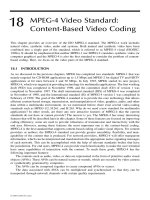
horizontally, vertically, or temporally. By

temporally

, we mean that the estimated displacement
vector can be passed to the pixel of the same spatial position within image planes in a temporally
neighboring frame. Figure 12.1 illustrates these three different types of recursion.

12.2 DESCENT METHODS

Consider a nonlinear real-valued function

z

of a vector variable ,
(12.2)
with

Œ



R

n

, where

R

n

represents the set of all

n

-tuples of real numbers. The question we face now
is how to find such a vector denoted by * that the function

z

is minimized. This is classified as
an unconstrained nonlinear programming problem.

12.2.1 F

IRST

-O

RDER

N

ECESSARY

C

ONDITIONS

According to the optimization theory, if

f

( ) has continuous first-order partial derivatives, then the
first-order necessary conditions that * has to satisfy are
(12.3)

FIGURE 12.1

Three types of recursions: (a) horizontal; (b) vertical; (c) temporal.
v
x
zfx=
()
v
,
v
x
v
x
v
x
v
x
—
()
=fx
v
*
,0

© 2000 by CRC Press LLC

where

—

denotes the gradient operation with respect to evaluated at *. Note that whenever there
is only one vector variable in the function

z

to which the gradient operator is applied, the sign

—

would remain without a subscript, as in Equation 12.3. Otherwise, i.e., if there is more than one
vector variable in the function, we will explicitly write out the variable, to which the gradient
operator is applied, as a subscript of the sign

—

. In the component form, Equation 12.3 can be
expressed as
(12.4)

12.2.2 S

ECOND

-O

RDER

S

UFFICIENT

C

ONDITIONS

If

F

( ) has second-order continuous derivatives, then the second-order sufficient conditions for

F

( *) to reach the minimum are known as
(12.5)
and
(12.6)
where

H

denotes the Hessian matrix and is defined as follows.
. (12.7)

We can thus see that the Hessian matrix consists of all the second-order partial derivatives of

f

with
respect to the components of . Equation 12.6 means that the Hessian matrix

H

is positive definite.

12.2.3 U

NDERLYING

S

TRATEGY

Our aim is to derive an iterative procedure for the minimization. That is, we want to find a sequence
(12.8)
such that
(12.9)
and the sequence converges to the minimum of

f

( ),

f

( *).
v
x
v
x
∂
()
∂
=
∂
()
∂
=
∂
()
∂
=
Ï
Ì
Ô
Ô
Ô
Ô
Ó
Ô
Ô
Ô
Ô
fx

x
fx
x
fx
x
n
v
v
M
v
1
2
0
0
0.
v
x
v
x
—
()
=fx
v
*
0
H
v
x
*
,

()
> 0
H
v
vv
L
v
vv
L
v
MMMM
vv
L
v
x
fx
x
fx
xx
fx
xx
fx
xx
fx
x
fx
xx
fx
xx
fx

xx
f
n
n
nn
()
=
∂
()
∂
∂
()
∂∂
∂
()
∂∂
∂
()
∂∂
∂
()
∂
∂
()
∂∂
∂
()
∂∂
∂
()

∂∂
∂
2
2
1
2
12
2
1
2
21
2
2
2
2
2
2
1
2
2
2
xx
x
n
()
∂
È
Î
Í
Í

Í
Í
Í
Í
Í
Í
˘
˚
˙
˙
˙
˙
˙
˙
˙
˙
2
v
x
vvv
L
v
Lxxx x
n012
,,,,,,
fx fx fx fx
n
vvv
L
v

L
012
()
>
()
>
()
>>
()
>
v
x
v
x

© 2000 by CRC Press LLC

A fundamental underlying strategy for almost all the descent algorithms (Luenberger, 1984) is
described next. We start with an initial point in the space; we determine a direction to move
according to a certain rule; then we move along the direction to a relative minimum of the function

z

. This minimum point becomes the initial point for the next iteration.
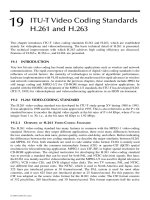
This strategy can be better visualized using a 2-D example, shown in Figure 12.2. There, =
(

x

1

,

x

2

)

l

. Several closed curves are referred to as

contour



curves

or

level curves

. That is, each of
the curves represents
(12.10)
with

c

being a constant.
Assume that at the

k

th iteration, we have a guess:

k

. For the (

k

+ l)th iteration, we need to
• Find a search direction, pointed by a vector

k

;
• Determine an optimal step size

a

k

with

a

k

> 0,
such that the next guess

k

+1

is
(12.11)
and

k

+1

satisfies

f

(

k

) >

f

(

k

+1

).
In Equation 12.11,

k

can be viewed as a prediction vector for

k

+1

, while

a

kk

an update
vector,

k

. Hence, using the Taylor series expansion, we can have
(12.12)
where

·

s

,

t

Ò

denotes the inner product between vectors and

Æ

t

; and

e

represents the higher-order
terms in the expansion. Consider that the increment of

a

kk

is small enough and, thus,

e

can be
ignored. From Equation 12.10, it is obvious that in order to have

f

(

k

+1

) <

F

(

k

) we must have

·—

f

(

k

),

a

kk



Ò

< 0. That is,
(12.13)

FIGURE 12.2

Descent



method.
v
x
fx x c
12
,,
()
=
v
x
v

w
v
x
vv
r
xx
kkkk+
=+
1
aw
v
x
v
x
v
x
v
x
v
x
v
w
v
v
fx fx fx
kk kkk
vv v
r
+
()

=
()
+—
()
+
1
,,aw e
v
s
v
w
v
x
v
x
v
x
v
w
fx fx fx
kk kkk
vv v
v
+
()
<
()
fi—
()
<

1
0,.aw
© 2000 by CRC Press LLC
Choosing a different update vector, i.e., the product of the
k
vector and the step size a
k
, results
in a different algorithm in implementing the descent method.
In the same category of the descent method, a variety of techniques have been developed. The
reader may refer to Luenberger (1984) or the many other existing books on optimization. Two
commonly used techniques of the descent method are discussed below. One is called the steepest
descent method, in which the search direction represented by the vector is chosen to be opposite
to that of the gradient vector, and a real parameter of the step size a
k
is used; the other is the
Newton–Raphson method, in which the update vector in estimation, determined jointly by the
search direction and the step size, is related to the Hessian matrix, defined in Equation 12.7. These
two techniques are further discussed in Sections 12.2.5 and 12.2.6, respectively.
12.2.4 CONVERGENCE SPEED
Speed of convergence is an important issue in discussing the descent method. It is utilized to
evaluate the performance of different algorithms.
Order of Convergence — Assume a sequence of vectors {
k
}, with k = 0, 1, L, •, converges to
a minimum denoted by *. We say that the convergence is of order p if the following formula
holds (Luenberger, 1984):
(12.14)
where p is positive, denotes the limit superior, and | | indicates the magnitude or norm of a
vector argument. For the two latter notions, more descriptions follow.

The concept of the limit superior is based on the concept of supremum. Hence, let us first
discuss the supremum. Consider a set of real numbers, denoted by Q, that is bounded above. Then
there must exist a smallest real number o such that for all the real numbers in the set Q, i.e., q Œ
Q, we have q £ o. This real number o is referred to as the least upper bound or the supremum of
the set Q, and is denoted by
(12.15)
Now turn to a real bounded above sequence r
k
, k = 0,1,L,•. If s
k
= sup{r
j
: j ≥ k}, then the sequence
{s
k
} converges to a real number s*. This real number s* is referred to as the limit superior of the
sequence {r
k
} and is denoted by
(12.16)
The magnitude or norm of a vector , denoted by ΈΈ, is defined as
(12.17)
where ·s, tÒ is the inner product between the vector and . Throughout this discussion, when we
say vector we mean column vector. (Row vectors can be handled accordingly.) The inner product
is therefore defined as
(12.18)
v
w
v
w

v
x
v
x
0
1
£
-
-
<•
Æ•
+
lim ,
*
*
k
k
k
p
xx
xx
vv
vv
lim
sup : sup .qq Q q
qQ
Œ
{}
()
Œ

or
lim .
k
k
r
Æ•
()
v
x
v
x
vvv
xxx= ,,
v
s
v
t
v
v
v
v
st st
T
,,,=
© 2000 by CRC Press LLC
with the superscript T indicating the transposition operator.
With the definitions of the limit superior and the magnitude of a vector introduced, we are now
in a position to understand easily the concept of the order of convergence defined in Equation 12.14.
Since the sequences generated by the descent algorithms behave quite well in general (Luenberger,
1984), the limit superior is rarely necessary. Hence, roughly speaking, instead of the limit superior,

the limit may be used in considering the speed of convergence.
Linear Convergence — Among the various orders of convergence, the order of unity is of
importance, and is referred to as linear convergence. Its definition is as follows. If a sequence {
k
},
k = 0,1,L,•, converges to * with
(12.19)
then we say that this sequence converges linearly with a convergence ratio g. The linear convergence
is also referred to as geometric convergence because a linear convergent sequence with convergence
ratio g converges to its limit at least as fast as the geometric sequences cg
k
, with c being a constant.
12.2.5 STEEPEST DESCENT METHOD
The steepest descent method, often referred to as the gradient method, is the oldest and simplest
one among various techniques in the descent method. As Luenberger pointed out in his book, it
remains the fundamental method in the category for the following two reasons. First, because of
its simplicity, it is usually the first method attempted for solving a new problem. This observation
is very true. As we shall see soon, when handling the displacement estimation as a nonlinear
programming problem in the pel recursive technique, the first algorithm developed by Netravali
and Robbins is essentially the steepest descent method. Second, because of the existence of a
satisfactory analysis for the steepest descent method, it continues to serve as a reference for
comparing and evaluating various newly developed and more advanced methods.
Formula — In the steepest descent method,
k
is chosen as
(12.20)
resulting in
(12.21)
where the step size a
k

is a real parameter, and, with our rule mentioned before, the sign — here
denotes a gradient operator with respect to
k
. Since the gradient vector points to the direction
along which the function f( ) has greatest increases, it is naturally expected that the selection of
the negative direction of the gradient as the search direction will lead to the steepest descent of
f( ). This is where the term steepest descent originated.
Convergence Speed — It can be shown that if the sequence { } is bounded above, then the steepest
descent method will converge to the minimum. Furthermore, it can be shown that the steepest
descent method is linear convergent.
Selection of Step Size — It is worth noting that the selection of the step size a
k
has significant
influence on the performance of the algorithm. In general, if it is small, it produces an accurate
v
x
v
x
lim ,
*
*
k
k
k
xx
xx
Æ•
+
-
-

=<
vv
vv
1
1g
v
w
v
v
w=-—
()
fx
k
,
fx fx fx
kkkk
vv v
+
()
=
()
-—
()
1
a ,
v
x
v
x
v

x
v
x
© 2000 by CRC Press LLC
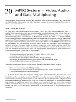
estimate of *. But a smaller step size means it will take longer for the algorithm to reach the
minimum. Although a larger step size will make the algorithm converge faster, it may lead to an
estimate with large error. This situation can be demonstrated in Figure 12.3. There, for the sake of
an easy graphical illustration, is assumed to be one dimensional. Two cases of too small (with
subscript 1) and too large (with subscript 2) step sizes are shown for comparison.
12.2.6 NEWTON-RAPHSON’S METHOD
The Newton–Raphson method is the next most popular method among various descent methods.
Formula — Consider
k
at the kth iteration. The k + 1th guess,
k+1
, is the sum of
k
and
k
,
(12.22)
where
k
is an update vector as shown in Figure 12.4. Now expand the
k+1
into the Taylor series
explicitly containing the second-order term.
(12.23)
where j denotes the higher-order terms, — the gradient, and H the Hessian matrix. If is small
enough, we can ignore the j. According to the first-order necessary conditions for

k+1
to be the
minimum, discussed in Section 12.2.1, we have
(12.24)
FIGURE 12.3 An illustration of effect of selection of step size on minimization performance. Too small a
requires more steps to reach x*. Too large a may cause overshooting.
FIGURE 12.4 Derivation of the
Newton–Raphson method.
v
x
v
x
v
x
v
x
v
x
v
v
vvv
xxv
kkk+
=+
1
,
v
v
v
x

fx fx fv Hx vv
kk k
vv v vvv
+
()
-
()
+— +
()
+
1
1
2
,,,j
v
v
v
x
—+
()
=—
()
+
()
=
v
vv v vv
v
kkk
fx v fx x vH 0,

© 2000 by CRC Press LLC
where —
v
denotes the gradient operator with respect to . This leads to
(12.25)
The Newton–Raphson method is thus derived below.
(12.26)
Another loose and intuitive way to view the Newton–Raphson method is that its format is similar
to the steepest descent method, except that the step size a
k
is now chosen as H
–1
(
k
), the inverse
of the Hessian matrix evaluated at
k
.
The idea behind the Newton–Raphson method is that the function being minimized is approx-
imated locally by a quadratic function and this quadratic function is then minimized. It is noted
that any function will behave like a quadratic function when it is close to the minimum. Hence,
the closer to the minimum, the more efficient the Newton–Raphson method. This is the exact
opposite of the steepest descent method, which works more efficiently at the beginning, and less
efficiently when close to the minimum. The price paid with the Newton–Raphson method is the
extra calculation involved in evaluating the inverse of the Hessian matrix at
k
.
Convergence Speed — Assume that the second-order sufficient conditions discussed in
Section 12.2.2 are satisfied. Furthermore, assume that the initial point
0

is sufficiently close to
the minimum *. Then it can be shown that the Newton–Raphson method converges with an order
of at least two. This indicates that the Newton–Raphson method converges faster than the steepest
descent method.
Generalization and Improvements — In Luenberger (1984), a general class of algorithms is
defined as
(12.27)
where G denotes an n ¥ n matrix, and a
k
a positive parameter. Both the steepest descent method
and the Newton–Raphson method fall into this framework. It is clear that if G is an n ¥ n identical
matrix I, this general form reduces to the steepest descent method. If G = H and a = 1 then this
is the Newton–Raphson method.
Although it descends rapidly near the solution, the Newton–Raphson method may not descend
for points far away from the minimum because the quadratic approximation may not be valid there.
The introduction of the a
k
, which minimizes f, can guarantee the descent of f at the general points.
Another improvement is to set G = [z
k
I + H(
k
)]
–1
with z ≥ 0. Obviously, this is a combination of
the steepest descent method and the Newton–Raphson method. Two extreme ends are that the
steepest method (very large z
k
) and the Newton–Raphson method (z
k

= 0). For most cases, the
selection of the parameter z
k
aims at making the G matrix positive definite.
12.2.7 OTHER METHODS
There are other gradient methods such as the Fletcher–Reeves method (also known as the conjugate
gradient method) and the Fletcher–Powell–Davidon method (also known as the variable metric
method). Readers may refer to Luenberger (1984) or other optimization text.
12.3 THE NETRAVALI–ROBBINS PEL RECURSIVE ALGORITHM
Having had an introduction to some basic nonlinear programming theory, we now turn to the pel
recursive technique in displacement estimation from the perspective of the descent methods. Let
v
v
vvv
vxfx
kk
=-
()
—
()
-
H
1
.
fx fx x fx
kk kk
vv vv
+-
()
=

()
-
()
—
()
11
H .
v
x
v
x
v
x
v
x
v
x
vv v
xx Gfx
kkk k+
=- —
()
1
a ,
v
x
© 2000 by CRC Press LLC
us take a look at the first pel recursive algorithm, the Netravali–Robbins pel recursive algorithm.
It actually estimates displacement vectors using the steepest descent method to minimize the squared
DFD. That is,

(12.28)
where — DFD
2
(x, y,
k
) denotes the gradient of DFD
2
with respect to evaluated at
k
, the
displacement vector at the kth iteration, and a is positive. This equation can be further written as
(12.29)
A a result of Equation 12.1, the above equation leads to
(12.30)
where —
x, y
means a gradient operator with respect to x and y. Netravali and Robbins (1979) assigned
a constant of
1
/
1024
to a, i.e.,
1
/
1024
.
12.3.1 INCLUSION OF A NEIGHBORHOOD AREA
To make displacement estimation more robust, Netravali and Robbins considered an area for
evaluating the DFD
2

in calculating the update term. More precisely, they assume the displacement
vector is constant within a small neighborhood W of the pixel for which the displacement is being
estimated. That is,
(12.31)
where i represents an index for the ith pixel (x, y) within W, and w
i
is the weight for the ith pixel
in W . All the weights satisfy the following two constraints.
(12.32)
(12.33)
This inclusion of a neighborhood area also explains why pel recursive technique is classified into
the category of region-matching techniques as we discussed at the beginning of this chapter.
12.3.2 INTERPOLATION
It is noted that interpolation will be necessary when the displacement vector components d
x
and
d
y
are not integer numbers of pixels. A bilinear interpolation technique is used by Netravali and
Robbins (1979). For the bilinear interpolation, readers may refer to Chapter 10.
12.3.3 SIMPLIFICATION
To make the proposed algorithm more efficient in computation, Netravali and Robbins also proposed
simplified versions of the displacement estimation and interpolation algorithms in their paper.
vv v
v
d d DFD x y d
kk
d
k+
=- —

()
12
1
2
a ,, ,
v
d
v
d
v
d
v
d
vv v v
v
d d DFD x y d DFD x y d
kk k
d
k+
=-
()
—
()
1
a ,, ,, .
vv v
d d DFD x y d f x d y d
kk k
xy n x y
+

-
=-
()
—
()
1
1
a ,, , ,
,
vv v
v
d d w DFD x y d
kk
d
i
k
ixy
+
Œ
=-—
()
Â
12
1
2
a ,,; ,
,,,W
w
w
i

l
i
≥
=
Ï
Ì
Ô
Ó
Ô
Œ
Â
0
1
W
.
© 2000 by CRC Press LLC
One simplified version of the Netravali and Robbins algorithm is as follows:
(12.34)
where sign{s} = 0, 1, –1, depending on s = 0, s > 0, s < 0, respectively, while the sign of a vector
quantity is the vector of signs of its components. In this version the update vectors can only assume
an angle which is an integer multiple of 45°. As shown in Netravali and Robbins (1979), this version
is effective.
12.3.4 PERFORMANCE
The performance of the Netravali and Robbins algorithm has been evaluated using computer
simulation (Netravali and Robbins, 1979). Two video sequences with different amounts and different
types of motion are tested. In either case, the proposed pel recursive algorithm displays superior
performance over the replenishment algorithm (Mounts, 1969; Haskell, 1979), which was discussed
briefly in Chapter 10. The Netravali and Robbins algorithm achieves a bit rate which is 22 to 50%
lower than that required by the replenishment technique with the simple frame difference prediction.
12.4 OTHER PEL RECURSIVE ALGORITHMS

The progress and success of the Netravali and Robbins algorithm stimulated great research interests
in pel recursive techniques. Many new algorithms have been developed. Some of them are discussed
in this section.
12.4.1 THE BERGMANN ALGORITHM (1982)
Bergmann modified the Netravali and Robbins algorithm by using the Newton–Raphson method
(Bergmann, 1982). In doing so, the following difference between the fundamental framework of
the descent methods discussed in Section 12.2 and the minimization problem in displacement
estimation discussed in Section 12.3 need to be noticed. That is, the object function f( ) discussed
in Section 12.2 now becomes DFD
2
(x, y, ). The Hessian matrix H, consisting of the second-order
partial derivatives of the f( ) with respect to the components of now become the second-order
derivatives of DFD
2
with respect to d
x
and d
y
. Since the vector is a 2-D column vector now, the
H matrix is hence a 2 ¥ 2 matrix. That is,
(12.35)
As expected, the Bergmann algorithm (1982) converges to the minimum faster than the steepest
descent method since the Newton–Raphson method converges with an order of at least two.
12.4.2 THE BERGMANN ALGORITHM (1984)
Based on the Burkhard and Moll algorithm (Burkhard and Moll, 1979), Bergmann developed an
algorithm that is similar to the Newton–Raphson algorithm. The primary difference is that an
average of two second-order derivatives is used to replace those in the Hessian matrix. In this sense,
it can be considered as a variation of the Newton–Raphson algorithm.
vv v
d d sign DFD x d sign f x d y d

kk k
xy n x y
+
-
=-
()
{}
—
()
{}
1
1
a ,, , ,
,
v
x
v
d
v
x
v
x
v
d
H =
∂
()
∂
∂
()

∂∂
∂
()
∂∂
∂
()
∂
È
Î
Í
Í
Í
Í
Í
˘
˚
˙
˙
˙
˙
˙
22
2
22
22 22
2
DFD x y d
d
DFD x y d
dd

DFD x y d
dd
DFD x y d
d
xxy
yx y
,, ,,
,, ,,
.
vv
vv
© 2000 by CRC Press LLC
12.4.3 THE CAFFORIO AND ROCCA ALGORITHM
Based on their early work (Cafforio and Rocca, 1975), Cafforio and Rocca proposed an algorithm
in 1982, which is essentially the steepest descent method. That is, the step size a is defined as
follows (Cafforio and Rocca, 1982):
(12.36)
with h
2
= 100. The addition of h
2
is intended to avoid the problem that would have occurred in a
uniform region where the gradients are very small.
12.4.4 THE WALKER AND RAO ALGORITHM
Walker and Rao developed an algorithm based on the steepest descent method (Walker and Rao,
1984; Tekalp, 1995), and also with a variable step size. That is,
(12.37)
where
(12.38)
It is observed that this step size is variable instead of being a constant. Furthermore, this variable

step size is reverse proportional to the norm square of the gradient of f
n–1
(x – d
x
, y – d
y
) with
respect to x, y. That means this type of step size will be small in the edge or rough area, and will
be large in the relatively smooth area. These features are desirable.
Although it is quite similar to the Cafforio and Rocca algorithm, the Walker and Rao algorithm
differs in the following two aspects. First, the a is selected differently. Second, implementation of
the algorithm is different. For instance, instead of putting an h
2
in the denominator of a, the Walker
and Rao algorithm uses a logic.
As a result of using the variable step size a, the convergence rate is improved substantially.
This implies fast implementation and accurate displacement estimation. It was reported that usually
one to three iterations are able to achieve quite satisfactory results in most cases.
Another contribution is that the Walker and Rao algorithm eliminates the need to transmit
explicit address information to bring out higher coding efficiency.
12.5 PERFORMANCE COMPARISON
A comprehensive survey of various algorithms using the pel recursive technique can be found in
a paper by Musmann, Pirsch, and Grallert (1985). There, two performance features are compared
among the algorithms. One is the convergence rate and hence the accuracy of displacement
estimation. The other is the stability range. By stability range, we mean a range starting from which
an algorithm can converge to the minimum of DFD
2
, or the true displacement vector.
Compared with the Netravali and Robbins algorithm, those improved algorithms discussed in
the previous section do not use a constant step size, thus providing better adaptation to local image

a
h
=
—
()
+
-
1
1
2
2
fxdyd
nxy
,
,
a=
—
()
-
1
2
1
2
fxdyd
nxy
,
,
—
()
=

∂
()
∂
Ê
Ë
Á
Á
ˆ
¯
˜
˜
+
∂
()
∂
Ê
Ë
Á
Á
ˆ
¯
˜
˜
-

fxdyd
fxdyd
d
fxdyd
d

nxy
nxy
x
nxy
y
1
2
1
2
1
2
,
,,
.
© 2000 by CRC Press LLC
statistics. Consequently, they achieve a better convergence rate and more accurate displacement
estimation. According to Bergmann (1984) and Musmann et al. (1985), the Bergmann algorithm
(1984) performs best among these various algorithms in terms of convergence rate and accuracy.
According to Musmann et al. (1985), the Newton–Raphson algorithm has a relatively smaller
stability range than the other algorithms. This agrees with our discussion in Section 12.2.2. That
is, the performance of the Newton–Raphson method improves when it works in the area close to
the minimum. The choice of the initial guess, however, is relatively more restricted.
12.6 SUMMARY
The pel recursive technique is one of three major approaches to displacement estimation for motion
compensation. It recursively estimates displacement vectors in a pixel-by-pixel fashion. There are
three types of recursion: horizontal, vertical, and temporal. Displacement estimation is carried out
by minimizing the square of the displaced frame difference (DFD). Therefore, the steepest descent
method and the Newton–Raphson method, the two most fundamental methods in optimization,
naturally find their application in pel recursive techniques. The pioneering Netravali and Robbins
algorithm and several other algorithms such as the Bergmann (1982), the Cafforio and Rocca, the

Walker and Rao, and the Bergmann (1984) are discussed in this chapter. They can be classified
into one of two categories: the steepest-descent-based algorithms or the Newton–Raphson-based
algorithms. Table 12.1 contains a classification of these algorithms.
Note that the DFD can be evaluated within a neighborhood of the pixel for which a displacement
vector is being estimated. The displacement vector is assumed constant within this neighborhood.
This makes the displacement estimation more robust against various noises.
Compared with the replenishment technique with simple frame difference prediction (the first
real interframe coding algorithm), the Netravali and Robbins algorithm (the first pel recursive
technique) achieves much higher coding efficiency. Specifically, a 22 to 50% savings in bit rate
has been reported for some computer simulations. Several new pel recursive algorithms have made
further improvements in terms of the convergence rate and the estimation accuracy through replace-
ment of the fixed step size utilized in the Netravali and Robbins algorithm, which make these
algorithms more adaptive to the local statistics in image frames.
12.7 EXERCISES
12-1. What is the definition of the displaced frame difference? Justify Equation 12.1.
12-2. Why does the inclusion of a neighborhood area make the pel recursive algorithm more
robust against noise?
12-3. Compare the performance of the steepest descent method with that of the Newton–Raph-
son method.
TABLE 12.1
Classification of Several Pel Recursive Algorithms
Algorithms
Category I
Steepest Descent Based
Category II
Newton–Raphson Based
Netravali and Robbins Steepest descent
Bergmann (1982) Newton–Raphson
Walker and Rao Variation of steepest descent
Cafforio and Rocca Variation of steepest descent

Bergmann (1984) Variation of Newton–Raphson
© 2000 by CRC Press LLC
12-4. Explain the function of h
2
in the Cafforio and Rocca algorithm.
12-5. What is the advantage you expect to have from the Walker and Rao algorithm?
12-6. What is the difference between the Bergmann algorithm (1982) and the Bergmann
algorithm (1984)?
12-7. Why does the Newton–Raphson method have a smaller stability range?
REFERENCES
Bergmann, H. C. Displacement estimation based on the correlation of image segments, IEEE Proceedings of
International Conference on Electronic Image Processing, 215-219, York, U.K., July 1982.
Bergmann, H. C. Ein Schnell Konvergierendes Displacement-Schätzverfahrenfür die Interpolation von Fernse-
hbildsequenzen, Ph.D. dissertation, Technical University of Hannover, Hannover, Germany, February
1984.
Biemond, J., L. Looijenga, D. E. Boekee, and R. H. J. M. Plompen, A pel recursive Wiener-based displacement
estimation algorithm, Signal Processing, 13, 399-412, December 1987.
Burkhard, H. and H. Moll, A modified Newton–Raphson search for the model-adaptive identification of delays,
in Identification and System Parameter Identification, R. Isermann, Ed., Pergamon Press, New York,
1979, 1279-1286.
Cafforio, C. and F. Rocca, The differential method for image motion estimation, in Image Sequence Processing
and Dynamic Scene Analysis, T. S. Huang, Ed., Berlin, Germany: Springer-Verlag, New York, 1983, 104-124.
Haskell, B. G. Frame replenishment coding of television, a chapter in Image Transmission Techniques, W. K.
Pratt, Ed., Academic Press, New York, 1979.
Luenberger, D. G. Linear and Nonlinear Programming, Addison Wesley, Reading, MA, 1984.
Mounts, F. W. A video encoding system with conditional picture-element replenishment, Bell Syst. Tech. J.,
48(7), 2545-1554, 1969.
Musmann, H. G., P. Pirsch, and H. J. Grallert, Advances in picture coding, Proc. IEEE, 73(4), 523-548, 1985.
Netravali, A. N. and J. D. Robbins, Motion-compensated television coding: Part I, Bell Syst. Tech. J., 58(3),
631-670, 1979.

Tekalp, A. M. Digital Video Processing, Prentice-Hall, Englewood Cliffs, NJ, 1995.
Walker, D. R. and K. R. Rao, Improved pel-recursive motion compensation, IEEE Trans. Commun., COM-
32, 1128-1134, 1984.