Tài liệu Handbook of Machine Design P47 docx

CHAPTER
40
CAM
MECHANISMS
Andrzej
A.
Ol?dzki,
D.Sc.
f
Warsaw
Technical
University,
Poland
SUMMARY
/
40.1
40.1
CAM
MECHANISM
TYPES,
CHARACTERISTICS,
AND
MOTIONS
/
40.1
40.2
BASIC
CAM
MOTIONS
/
40.6

40.3
LAYOUT
AND
DESIGN;
MANUFACTURING
CONSIDERATIONS
/
40.17
40.4
FORCE
AND
TORQUE
ANALYSIS
/
40.22
40.5
CONTACT
STRESS
AND
WEAR:
PROGRAMMING
/
40.25
REFERENCES
/
40.28
SUMMARY
This chapter addresses
the
design

of cam
systems
in
which
flexibility
is not a
consid-
eration. Flexible, high-speed
cam
systems
are too
involved
for
handbook presenta-
tion. Therefore only
two
generic
families
of
motion, trigonometric
and
polynomial,
are
discussed. This covers most
of the
practical problems.
The
rules concerning
the
reciprocating motion

of a
follower
can be
adapted
to
angular
motion
as
well
as to
three-dimensional cams. Some material concerns circu-
lar-arc cams, which
are
still used
in
some
fine
mechanisms.
In
Sec.
40.3
the
equations
necessary
in
establishing basic parameters
of the cam are
given,
and the
important

problem
of
accuracy
is
discussed.
Force
and
torque analysis, return springs,
and
con-
tact
stresses
are
briefly
presented
in
Sees.
40.4
and
40.5, respectively.
The
chapter closes with
the
logic associated with
cam
design
to
assist
in
creating

a
computer-aided
cam
design program.
40.7
CAM
MECHANISM
TYPES,
CHARACTERISTICS,
AND
MOTIONS
Cam-and-follower
mechanisms,
as
linkages,
can be
divided into
two
basic groups:
1.
Planar
cam
mechanisms
2.
Spatial
cam
mechanisms
In a
planar
cam

mechanism,
all the
points
of the
moving links describe paths
in
par-
allel planes.
In a
spatial mechanism, that requirement
is not
fulfilled.
The
design
of
mechanisms
in the two
groups
has
much
in
common. Thus
the
fundamentals
of
pla-
nar
cam
mechanism design
can be

easily applied
to
spatial
cam
mechanisms, which
f
Prepared
while
the
author
was
Visiting Professor
of
Mechanical Engineering, Iowa State University,
Ames, Iowa.
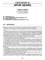
FIGURE
40.1
(a)
Planar
cam
mechanism
of the
internal-combustion-engine D-R-D-R type;
(b)
spatial
cam
mechanism
of the
16-mm
film

projector R-D-R type.
is
not the
case
in
linkages. Examples
of
planar
and
spatial mechanisms
are
depicted
in
Fig. 40.1.
Planar
cam
systems
may be
classified
in
four
ways:
(1)
according
to the
motion
of
the
follower—reciprocating
or

oscillating;
(2) in
terms
of the
kind
of
follower sur-
face
in
contact—for
example, knife-edged,
flat-faced,
curved-shoe,
or
roller;
(3) in
terms
of the
follower
motion—such
as
dwell-rise-dwell-return
(D-R-D-R),
dwell-
rise-return (D-R-R), rise-return-rise (R-R-R),
or
rise-dwell-rise
(R-D-R);
and (4) in
terms

of the
constraining
of the
follower—spring
loading (Fig.
40.1«)
or
positive
drive (Fig.
40.16).
Plate
cams acting with
four
different
reciprocating followers
are
depicted
in
Fig.
40.2
and
with oscillating followers
in
Fig. 40.3.
Further
classification
of
reciprocating followers distinguishes whether
the
cen-

terline
of the
follower stem
is
radial,
as in
Fig. 40.2,
or
offset,
as in
Fig. 40.4.
Flexibility
of the
actual
cam
systems requires,
in
addition
to the
operating
speed,
some data concerning
the
dynamic
properties
of
components
in
order
to

find
dis-
crepancies between rigid
and
deformable
systems. Such data
can be
obtained
from
dynamic
models. Almost every actual
cam
system can, with certain simplifications,
be
modeled
by a
one-degree-of-freedom
system, shown
in
Fig. 40.5, where
m
e
FIGURE
40.2 Plate cams with reciprocating followers.
FIGURE
40.3
Plate
cams
with
oscillating

followers.
denotes
an
equivalent mass
of the
system,
k
e
equals equivalent
stiffness,
and s and y
denote, respectively,
the
input (coming
from
the
shape
of the cam
profile)
and the
output
of the
system.
The
equivalent mass
m
e
of the
system
can be

calculated
from
the
following equation, based
on the
assumption that
the
kinetic energy
of
that mass
equals
the
kinetic energy
of all the
links
of the
mechanism:
1
^?
YHjV]
1
^
I
1
W]
m
e
=
L—^-^L-^T
Z

=
I
A
i
=
1
*
where
ra, =
mass
of
link
i
VI
=
linear velocity
of
center
of
mass
of
z'th
link
Ii
=
moment
of
inertia about center
of
mass

for
/th
link
co,
=
angular velocity
of
ith
link
5
=
input velocity
The
equivalent
stiffness
k
e
can be
found
from
direct measurements
of the
actual
system
(after
a
known force
is
applied
to the

last link
in the
kinematic chain
and the
displacement
of
that link
is
measured), and/or
by
assuming that
k
e
equals
the
actual
stiffness
of the
most flexible link
in the
chain.
In the
latter case,
k
e
can
usually
be
cal-
culated

from
data
from
the
drawing, since
the
most
flexible
links usually have
a
sim-
ple
form
(for example,
a
push
rod in the
automotive
cam of
Fig.
40.16c).
In
such
a
FIGURE
40.4
Plate
cam
with
an

offset
recip-
rocating
roller
follower.
FIGURE
40.5
The
one-degree-of-freedom
cam
system
model.
model,
the
natural frequency
of the
mass
m
e
is
co
e
=
\/k
e
lm
e
and
should
be

equal
to
the
fundamental frequency
co
n
of the
actual system.
The
motion
of the
equivalent mass
can be
described
by the
differential equation
m
e
y
+
k
e
(y
-s)
=
Q
(40.1)
where
y
denotes acceleration

of the
mass
m
e
.
Velocity
s
and
acceleration
s
at the
input
to the
system
are
ds
ds J0 ,
/A
^^
s
=
—
= — — =
s'co
(40.2)
dt
dQ
dt
v
'

and
d
,
d?'
,
Jco
d«'
JG
J=-T
5
CO=
(0 +
5
-—-
=
a5
—-
CO+
S
OC
Jr
Jt
Jf
(40.3)
=
s"co
2
+
s'cc
where

6 =
angular displacement
of cam
a =
angular acceleration
of cam
s
'=
ds/
JG,
the
geometric
velocity
s
"=
ds
7
JG
=
J
2
^JG
2
,
the
geometric acceleration
When
the cam
operates
at

constant nominal speed
co
=
CO
0
,
Jco/Jf
=
oc
=
O and Eq.
(40.3) simplifies
to
s
=
s"(*i
(40.4)
The
same expressions
can be
used
for the
actual velocity
y and for the
actual accel-
eration
y at the
output
of the
system. Therefore

y
=
y'(Q
(40.5)
y
=
y"<i?
+
y'a
(40.6)
or
y=y"a?o
co =
CO
0
=
constant (40.7)
Substituting
Eq.
(40.7) into
Eq.
(40.1)
and
dividing
by
k
e
gives
^
d

y
"
+y
=
s
(40.8)
where
[i
d
=
(m
e
/A:
e
)cOo,
the
dynamic factor
of the
system.
Tesar
and
Matthew [40.10]
classify
cam
systems
by
values
of
(i
rf

,
and
their recom-
mendations
for the cam
designers, depending
on the
value
of
JLI^,
are as
follows:
[i
d
=
10~
6
(for low-speed systems; assume
s = y)
[i
d
=
10"
4
(for medium-speed systems;
use
trigonometric, trapezoidal motion specifi-
cations, and/or similar ones; synthesize
cam at
design

speed
co
=
CO
0
,
use
good manu-
facturing
practices
and
investigate distortion
due to
off-speed operations)
(i
rf
=
10~
2
(for high-speed systems;
use
polynomial motion specification
and
best
available manufacturing techniques)
FIGURE 40.6 Types
of
follower
motion.
In all the

cases, increasing
k
e
and
reducing
m
e
are
recommended, because
it
reduces
ji
rf
.
There
are two
basic phases
of the
follower motion,
rise
and
return. They
can be
combined
in
different
ways, giving types
of
cams classifiable
in

terms
of the
type
of
follower
motion,
as in
Fig. 40.6.
For
positive drives,
the
symmetric acceleration curves
are to be
recommended.
For cam
systems with spring restraint,
it is
advisable
to use
unsymmetric curves
because they allow smaller springs. Acceleration curves
of
both
the
symmetric
and
unsymmetric
types
are
depicted

in
Fig. 40.7.
FIGURE 40.7
Acceleration
diagrams: (a),
(b)
spring loading;
(c),
(d)
positive
drive.
40.2
BASICCAMMOTIONS
Basic
cam
motions consist
of two
families:
the
trigonometric
and the
polynomial.
40.2.1
Trigonometric
Family
This
family
is of the
form
s

"=
C
0
+
C
1
sin
00
+
C
2
cos
bQ
(40.9)
where
C
0
,
C
1
,
a,
and b are
constants.
For the
low-speed systems where
\i
d
<
10"

4
,
we can
construct
all the
necessary dia-
grams,
symmetric
and
unsymmetric,
from
just
two
curves:
a
sine curve
and a
cosine
curve.
Assuming
that
the
total rise
or
return motion
S
0
occurs
for an
angular displace-

ment
of the cam 0 =
p
0
,
we can
partition acceleration curves into
i
separate segments,
where
/
=
1,2,3,
with subtended angles
P
1
,
p
2
,
P
3
,
so
that
P
1
+
P
2

+
P
3
+ - =
Po-
The sum of
partial
lifts
S
1
,
S
2
,
S
3
,
in the
separate segments should
be
equal
to the
total rise
or
return
S
0
:
^i
+

S
2
+
S
3
+
—
=
SQ.
If a
dimensionless description
0/p of cam
rotation
is
introduced into
a
segment,
we
will
have
the
value
of
ratio
0/p
equal
to
zero
at the
beginning

of
each segment
and
equal
to
unity
at the end of
each segment.
All the
separate segments
of the
acceleration curves
can be
described
by
equa-
tions
of the
kind
s"=Asin^
/1
=
^,1,2
(40.10)
P
2
or
s"=
A
cos^

(40.11)
where
A is the
maximum
or
minimum value
of the
acceleration
in the
individual
segment.
The
simplest case
is
when
we
have
a
positive drive with
a
symmetric acceleration
curve
(Fig.
40.7d).
The
complete rise motion
can be
described
by a set of
equations

/0 1
2710
\
„
27W
0
27C0
J=ffo
fe
-
&
sm
"T
J
5=
~F
sm
~T
(40.12)
,
S
0
(
-
2710
\
,„
4n
2
s

0
2710
^Tl
1
-
008
!-)
s
=
-p-
cos
T
The
last term
is
called geometric jerk
(s'
=
coY").
Traditionally, this motion
is
called
cycloidal
The
same equations
can be
used
for the
return motion
of the

follower.
It is
easy
to
prove that
^return
~
^O
~~
^rise
$
return
~
~$
rise
(40.13)
v'
—
-v'
?'"——?'"
1
^
return
3
rise
J
return
1
^
rise

FIGURE 40.8 Trigonometric standard
follower
motions (according
to the
equation
of
Table 40.1,
for c = d =
O).
All the
other acceleration curves, symmetric
and
unsymmetric,
can be
constructed
from
just
four
trigonometric standard
follower
motions. They
are
denoted
further
by
the
numbers
1
through
4

(Fig. 40.8).
These
are
displayed
in
Table 40.1.
Equations
in
Table 40.1
can be
used
to
represent
the
different
segments
of a
fol-
lower's displacement diagram. Derivatives
of
displacement diagrams
for the
adja-
cent segments should match each other; thus several requirements must
be met in
order
to
splice them together
to
form

the
motion specification
for a
complete cam.
Motions
1
through
4
have
the
following
applications:
Motion
1 is for the
initial part
of a
rise motion.
Motion
2 is for the end
and/or
the
middle part
of a
rise motion
and the
initial part
of
a
return motion.
The

value
c is a
constant, equal
to
zero only
in
application
to
the end
part
of a
rise
motion.
Motion
3 is for the end
part
of a
rise motion and/or
the
initial
or
middle part
of a
return motion.
The
value
d is a
constant, equal
to
zero only

in
application
to the
initial
part
of a
return motion.
Motion
4 is for the end
part
of a
return motion.
The
procedure
of
matching
the
adjacent
segments
is
best understood through
examples.
Example
1.
This
is an
extended version
of
Example
5-2

from
Shigley
and
Uicker
[40.8],
p.
229. Determine
the
motion specifications
of a
plate
cam
with
reciprocating
TABLE
40.1
Standard Trigonometric Follower Motions
Parameter
Motion
1
Motion
2
Motion
3
Motion
4
5
j,/V0
.
7r0\

.
vo
e
re
(e
i\
f e
i
*e\
T~
sm
T
S2
*
m
™"*
c
~n
53008
TF
+
^U"?
M
1
T-^
11
T
If
\P\
PlJ

2/3
2
P2
2^
3
\0
3
2/ V
0
4
TT
#4/
5'
Sj/.
7T^\
5
2
1T
*0
C
SjT
.
IfB
d
S
4
L
*6\
A
I

1
-""ft)
2fe
C
°
S
2ft
+
^
-2^
Wn
2ft
+
^
-id
1+C
°
S
£J
5*
tr5,
.
IT^
S
2
ir
2
.
*0
5

3
ir
2
TT^
TTS
4
.
ir0
W-
11
A'
~^
sm
%
-^'^
^r
sin
^
J^"
TT
2
^
1
TT^
J
2
*
3
TO
Si**

•
*0
T
2
S*
V0
1T
COS
^
-8^
C
°
S
%
8l
Sm
2^
7T
C
°
S
£
S
'
/1 -
O^

&•
- -
^

4
"Ur
}
2^
A
ft
^.
(L-t\
25,
£
_M
+
^
*"*U-
/
/J
1
ft
2ft
+
ft
**«.;**.
.»
-2*1

__a!
.»
_af
,"-2^
^

max
^j
S
min
-
^
*
™"
4j
g2
m
"
~
/Sj
FIGURE
40.9 Example
1: (a)
displacement diagram,
in; (b)
geometric velocity diagram, in/rad;
(c)
geomet-
ric
acceleration diagram,
in/rad
2
.
follower
and
return spring

for the
following
requirements:
The
speed
of the cam is
con-
stant
and
equal
to 150
r/min.
Motion
of the
follower consists
of six
segments (Fig.
40.9):
1.
Accelerated motion
to
s^
end
= 25
in/s (0.635 m/s)
2.
Motion with constant velocity
25
in/s, lasting
for

1.25
in
(0.03175
m) of
rise
3.
Decelerated
motion (segments
1 to 3
describe
rise of the
follower)
4.
Return motion
5.
Return motion
6.
Dwell, lasting
for t
>
0.085
s
The
total
lift
of the
follower
is 3 in
(0.0762
m).

Solution.
Angular velocity
CG
=
15071730
=
15.708 radians
per
second (rad/s).
The
cam
rotation
for
1.25
in of
rise
is
equal
to
p
2
=
1.25
mlS
2
=
1.25 in/1.592 in/rad
=
0.785
rad

-
45°, where
si =
25/15.708
-
1.592 in/rad.
The
following decisions
are
quite arbitrary
and
depend
on the
designer:
1. Use
motion
1;
then
S
1
= 0.5 in,
<
ax
-
0.057C/P
2
!
-
0.5jc/(0.628)
2

-
4
in/rad
2
(0.1016
m/rad
2
).
s"^
d
=
2(0.5)/pi;
so
P
1
-
1/1.592
=
0.628 rad,
or
36°.
2. For the
motion with constant velocity,
S
2
-1.592
in/rad (0.4044
m/rad);
S
2

=
1.25
in.
3.
Motion type
2:
S
3
=
S
2
=
1.25
in,
$3'^
=
s
3
7i/(2p
3
)
=
1.592 in/rad; therefore
p
3
=
1.257C/[2(1.592)]
-1.233
rad
=

71°,
^n
=
-(1.257i
2
)/[4(1.233)
2
]
= -2
in/rad
2
.
(Points
1
through
3
describe
the
rise motion
of the
follower.)
4.
Motion type
3:s4'
init
=s
4
7r
2
/(4p

2
)
= -2
in/rad
2
(the same value
as
that
of
s^),
s£
end
=
-7tt4/(2p
4
),
S
4
+
S
5
= 3 in.
5.
Motion type
4:
s
5
"
max
=

7W
5
/P
2
,
s
5
'i
nit
= -
s(
end
=
-2s
5
/fi
5
.
We
have here
the
four
unknowns
p
4
,
S
4
,
p

5
,
and
S
5
.
Assuming time
I
6
=
0.85
s for the
sixth segment
(a
dwell),
we can
find
(3
6
=
COf
6
=
15.708(0.08)
=
1.2566 rad,
or
72°.
Therefore
P

4
+
P
5
=
136°,
or
2.374
rad
(Fig. 40.9). Three other equations
are
S
4
+
S
5
=
3,s
4
n
2
/(4$)
= 2,
and
7cs
4
/(2p
4
)
=

2s
5
/p
5
.
From these
we can
derive
the
quadratic equation
in
p
4
.
0.696Pi
+
6.044p
4
-12
=
Q
Solving
it, we
find
p
4
=
1.665
848 rad
=

95.5°
and
p
5
=
40.5°. Since
S
4
Is
5
=
4p
4
/(7ip
5
)
=
3.000
76, it is
easy
to
find
that
S
5
=
0.75
in
(0.019
05 m) and

S
4
=
2.25
in
(0.057
15
m).
Maximum geometric acceleration
for the
fifth
segment
s
5
'
max
=
4.7
in/rad
2
(0.0254
m/rad
2
),
and the
border (matching) geometric velocity
s
4>end
=
s^

=
2.12
in/rad
(0.253 m/rad).
Example
2. Now let us
consider
a cam
mechanism with spring loading
of the
type
D-R-D-R (Fig.
40.70).
The
rise part
of the
follower motion might
be
constructed
of
three segments
(1,2,
and 3)
described
by
standard follower motions
1,2,
and 3
(Fig.
40.8).

The
values
of
constants
c and d in
Table 40.1
are no
longer zero
and
should
be
found
from
the
boundary conditions. (They
are
zero only
in the
motion case R-R-D,
shown
in
Fig.
40.Jb,
where there
is no
dwell between
the
rise
and
return motions.)

For a
given motion specification
for the
rise motion,
the
total follower stroke
S
0
,
and the
total angular displacement
of the cam
p
0
,
we
have eight unknowns:
P
1
,
Si,
P
2
,
$2,
Ps>
S
3
,
and

constants
c and d. The
requirements
of
matching
the
displacement
derivatives
will
give
us
only
six
equations; thus
two
more must
be
added
to get a
unique
solution.
Two
additional equations
can be
written
on the
basis
of two
arbi-
trary

decisions:
1. The
maximum value
of the
acceleration
in
segment
l,s"
tmsa
should
be
greater than
that
in
segment
2
because
of
spring loading.
So
s"
max
=
-as"
min
where
s^'mm
is
the
minimum

value
of the
second-segment acceleration
and a is any
assumed num-
ber, usually greater than
2.
2. The end
part
of the
rise (segment
3), the
purpose
of
which
is to
avoid
a
sudden
drop
in a
negative accelerative curve, should have
a
smaller duration than
the
basic
negative part (segment
2).
Therefore
we can

assume
any
number
b
(greater
than
5) and
write
p
2
=
&p
3
.The
following
formulas were
found
after
all
eight equa-
tions
for the
eight unknowns were solved simultaneously:
R
Po Q
_«
a
^~l
+
a +

alb
^'
1
S(I
+
*)
+
*
TC^
,_
4a
Sl
~
S
°
b
2
(n
+
4a)
+
4a(2a
+
l)
"
2
~
Sl
K
4a

Sa
2
53
"
"
1
TtZ)
2
C
~
Sl
nb
2
d =
2s
3
SQ
=
Si+
52
+c
+
S
3
We
can
assume practical values
for a and b
(say
a =

2,
b = 10) and
find
from
the
above
equations
the set of all the
parameters
(as
functions
of
S
0
and
p
0
)
necessary
to
form
the
motion specification
for the
rise motion
of the
follower
and the
shape
of the cam

profile.
The
whole
set of
parameters
is as
follows:
5j
=
0.272
198so
Pi
=
0.312
5p
0
s'
2
=
0.693
147*0
c =
0.027
726s
0
P
2
=
0.625p
0

*3
=
0.006931*o
d
=
2s
3
(always!)
p
3
=
0.0625po
These
can be
used
for
calculations
of the
table
s =
5(6),
which
is
necessary
for
manu-
facturing
a cam
profile.
For

such
a
table,
we use as a
rule increments
of 0
equal
to
about
1°
and
accuracy
of s up to 4 x
10~
5
in 1
micrometer
(um).
The
data
of
such
a
table
can be
easily used
for the
description
of
both

the
return motion
of the
follower
and a cam
profile,
providing
p
0
(return)
=
J3
0
(rise),
and the
acceleration diagram
for
the
return motion
is a
mirror image
of the
acceleration diagram
for the
rise motion.
Table 40.2
can be of
assistance
in
calculating

the
return portion
of the cam
profile.
The
column
s(return)
is the
same
as the
column
s(rise).
TABLE
40.2
Data
of
Rise
Motion
Used
for
Calculations
of
Return
Portion
of Cam
Profile
Rise Return
0(rise)
s(rise)
^(return)

^return)
O
O
20Q
+
&/-0
O
Bi
s,
2A>
+
&/-0/
J/
0o
^
0
20o
+
0</
— 0o
S
0
The
trigonometric acceleration diagram
for the
positive drive
was
described
at
the

beginning
of
this section
by Eq.
(40.12).
The
improved diagram (smaller maxi-
mum
values
of
acceleration
for the
same values
of
S
0
and
p
0
f
)
can be
obtained
if we
combine sine segments with segments
of
constant acceleration. Such
a
diagram,
called

a
modified
trapezoidal
acceleration
curve,
is
shown
in
Fig. 40.10. Segments
1,
3,
4, and 6 are the
sinusoidal type. Sections
2 and 5 are
with
s" =
constant.
It was
assumed
for
that diagram that
all the
sine segments take one-eighth
of the
total
angular displacement
p
0
of the cam
during

its
rise
motion.
The
first
half
of the
motion
has
three
segments.
The
equations
for the
first
segment
are O
<
0/p
0
<
1
^,
and so
f
The
maximum
acceleration
ratio
is

4.9/6.28.
FIGURE 40.10
A
modified
trapezoidal acceleration diagram.
S
0
-
/47C0
.
4710
\
,
2s'
Q
/
47c9\
S
= —
-;r~
-
Sin
—:—
S
=-r—
1-COS
——
271
V Po Po
/

Po V Po
/
(40.14)
„
0
SQ .
47T0
„,
^
4rc9
5
=871-rj
sm-r—
s
=
327T
-TJ
cos
——
Po
Po Po Po
For the
second segment,
we
have
1
A
<
0/p
0

<
%,
and so
,[
1
29
/9
IVl
5:=5o
~^;
+
ir
+47C
U~~^
L
2n
Po VPo
8/J
/
=
^[
2
+
8icg i)l
(40.15)
Po
L
\Po
o
/J

„
8ns'
0
,„
s=
~w
s
=0
The
relations
for the
third segment
are
3
A
<
9/P
0
<
%
([40.7]);
therefore,
J
TC

,9
1 .
I"
/0
2\11

J
=
^o

+
2(1+7C)
—
sin
UTC
—

[2
Po
27C
L VPo
8
/JJ
'-f{—Nt-I)Il
(40.16)
„
87K
0
'
.
r
/e
2\]
s
=
ir

sm
rte-8JJ
^"=-i
cos
h(M)]
where
J
0
'
=
s<J(2
+
n)
=
0.194
492^
0
.
Using
Eqs. (40.14) through (40.16)
for all
three segments,
we can
calculate
the s
values
for the
first
half
of the

rise motion, where
6/p
0
-
%
and s =
s
0
/2.
Since
the
neg-
ative
part
of the
acceleration diagram
is a
mirror image
of the
positive part,
it is
easy
to
calculate
the s
values
for the
second
half
of the

rise motion
from
the
data obtained
for
the
first
half.
The
necessary procedure
for
that
is
shown
in
Table 40.3.
The
proce-
dure concerns
the
case with
the
modified trapezoidal acceleration diagram,
but it
could
be
used
as
well
for all the

cases with symmetric acceleration diagrams
for the
rise motion.
For the
return motion
of the
follower, when
its
acceleration diagram
is
a
mirror image
of the
rise diagram,
we can use
again
the
technique shown
in
Table
40.2.
All the
calculations
can be
done simultaneously
by the
computer
after
a
simple

program
is
written.
TABLE
40.3
Data
of
First
Half
of
Rise
Motion
Used
for
Calculations
of
Second
Half
7
-
W
0
s y s
0
O 1
S
0
1
T/
Sj

1 -
7/
SQ
-
Si
6
1
S
1
=
s'
0
(*/2
-
l)/27r
i
S
0
-S
1
t
*
f
'
0
T'
1
2
]>
sj

!
T
Tj
S
°~
Sj
5
1
S
2
-
S
0
(^
-'
1/2»
+
x/4)
J
5
°~
52
i
S
2
I
S
0
-S
2

y
Sk 1 -
7*
So-Sk
4
k
'
:
'
:
:
:
S
3
=
S
0
/2
I
S
0
-
S
3
=
S
0
/2
I
All the

trigonometric curves
of
this section were calculated with finite values
of
jerk,
which
is of
great importance
for the
dynamic behavior
of the cam
mechanism.
An
example
of the
jerk diagram
is
given
in
Fig.
40.10.
The
jerk curve
;
was
plotted
by
using
the
dimensionless expression

/=
^
(4ai7)
This
form
of the
jerk description
can
also
be
used
to
compare properties
of
different
acceleration diagrams.
Segments
40.2.2
Polynomial Family
The
basic polynomial equation
is
Q
/
Q
\2
/ 0
\
3
5-C

0
+
C
1
-
+C
2
-
+C
3
-
+».
(40.18)
Po
\Po/
\Po/
with
constants
C/
depending
on
assumed initial
and
final
conditions.
This
family
is
especially
useful

in the
design
of
flexible
cam
systems, where values
of
the
dynamic
factor
are
U^
>
10~
2
.
Dudley (1947)
first
used polynomials
for the
syn-
thesis
of
flexible
systems,
and his
ideal later
was
improved
by

Stoddart [40.9]
in
application
to
automotive
cam
gears.
The
shape
factor
s of the cam
profile
can be
found
by
this method
after
a
priori
decisions
are
made about
the
motion
y of the
last link
in the
kinematic chain. Cams
of
that kind

are
called
poly
dyne
cams.
When
flexibility
of the
system
can be
neglected,
the
initial
and
final
conditions
([40.3],
[40.4],
and
[40.8])
might
be as
follows
(positive drive):
1.
Initial conditions
for
full-rise
motion
are

-|-
= 0 s =
0
s'
=
0
s"
=
0
Po
2.
Final (end) conditions
are
-|-
= 1 s =
s
0
s'
= 0
s"
=
Q
Po
The
first
and
second derivatives
of Eq.
(40.18)
are

/
=
C
1
+
2C
2
|
+
3C
3
(|)
2
+
4C
4
(|)
3
+

Po
\
Po
/
\
Po
/
(40.19)
9 / 9 V
^

=
2C
2
+
6C
3
-T-+
12C
4
-
+•••
Po
\Po/
Substituting
six
initial
and
final
conditions into Eqs.
(40.18)
and
(40.19)
and
solving
them simultaneously
for
unknowns
C
0
,

Ci,
C
2
,
C
3
,
C
4
,
and
C
5
,
we
have
I79\
3
/9V
/9
Vl
"My-
L
4r
a6
(id]
'-"SKiMiHi)I
'-S[HiMi)I
and for a
jerk

s'"
=
ds"ld§,
or
—SHHifl
FIGURE
40.11
Full-rise
3-4-5
polynomial
motion.
After
a
proper
set of
initial
and
final
conditions
is
established,
the
basic equation
[Eq.
(40.18)]
can be
used
for
describing
any

kind
of
follower motion with
an
unsym-
metric acceleration diagram.
Details
concerning
the
necessary procedure
can be
found
in
Rothbart
[40.7].
40.2.3
Other
Cam
Motions
The
basic
cam
motions described
in the
previous sections cover most
of the
routine
needs
of the
contemporary

cam
designer. However, sometimes
the
cost
of
manufac-
turing
the cam
profile
may be too
high
and the
dynamic properties
of the cam
motion
may not be
severe. This
is the
case
of
cams used
for
generating functions.
There
is a
very
effective
approach, described
by
Mischke [40.2], concerning

an
opti-
mum
design
of
simple eccentric cams. They
are
very inexpensive,
yet can be
used
even
for
generating very complicated functions.
This
is
called
the
polynomial 3-4-5, since powers
3,4,
and 5
remain
in the
displace-
ment equation.
It
provides
a
fairly
good diagram
for the

positive drives.
Equations
for the
full-return polynomial
are
^(return)
=
-sirise)
+
S
0
/'(return)
= -
/(rise)
(40.21)
/'(return)
=
-/'(rise)
/"(return)
=
-/"(rise)
All the
characteristic curves
of the
full-rise
3-4-5 polynomial
are
shown
in
Fig.

40.11.
They were generated
by the
computer
for
SQ
=
I
displacement unit (inches
or
cen-
timeters)
and
po
= 1
rad.
The
other approach, when
we are
interested
in
inexpensive cams,
is to use
circular-
arc
cams
or
tangent cams. They
are
still used

in
low-speed
diesel
IC
engines since
the
cost
of
their manufacture
is low
(compare with Fig. 40.15).
An
extensive review
of
these cams
can be
found
in
Rothbart
[40.7].
They were used quite frequently
in the
past when
the
speed
of
machines
was
low,
but

today they
are not
often recommended
because their dynamic characteristics
are
poor.
The
only exception
can be
made
for
fine-
or
light-duty mechanisms, such
as
those
of 8- and
16-mm
film
projectors,
where
circular-arc
cams
are
still widely used. Those cams
are
usually
of the
positive drive
kind,

where
the
breadth
of the cam is
constant.
The cam
drives
a
reciprocating fol-
lower
with
two flat
working surfaces
a
fixed
distance apart, which contact
opposite
sides
of the
cam.
The
constant-breadth
cam is
depicted
in
Fig. 40.12.
For
given values
of
radius

p,
total angle
of cam
rotation
(3
0
,
and
total
lift
of the
follower
% the
basic dimensions
of
the cam can be
found
from
the
relations
([40.1I])
P-
b(Sp
+ P)
„
(Af\^\
K
1
——
r-Ki-So

(4U.zz;
FIGURE
40.12
Constant-breadth
circular-arc
cam.
where
b = cos
0.25(3
0
/cos
0.75p
0
.
Cam
motions
for
full
rise
(O
>
6
>
P
0
)
are
described
in
Table 40.4. Such cams

are
symmetric; therefore,
p
0
(rise)
=
p
0
(return),
and the two
dwells
p
rfl
and
p
rf2
are
the
same
and
equal
to
180°
-
J3
0
.
Table 40.4
can
also

be
used
for
calculation
of
full-return
motion. Dimensions
of the cam
(Ri)
and
maximum values
of
the
acceleration increase with
a
decrease
in
p
0
.
Acceleration diagrams
for
differ-
ent
values
of
P
0
are
shown

in
Fig. 40.13.
TABLE
40.4 Basic
Equations
for a
Constant-Breadth
Circular-Arc
Cam,
Using
A =
R
1
- p
Parameter
O
<
6
<//V2
/3
0
/2
<
B
<
/J
0
s
A(I
- cos

S)
A cos
(0o
—
B)
—
(r — p)
s
f
A sin
6
A sin
(0
0
— 0)
s"
A cos 0 -A cos
(fa
-
B)
s"'
-A
sin
0f
-A
sin
(0
0
-
0)f

t
Both
equations
are
valid,
however,
only
inside
the
partitions.
For 0 = 0,
f}
Q
/2,
and
00,
S"
->
oo.
FIGURE
40.13 Acceleration diagrams.
40.3 LAYOUT
AND
DESIGN; MANUFACTURING
CONSIDERATIONS
The cam
profile
is an
inner envelope
of the

working surface
of the
follower. After
the
displacement diagram
is
determined,
the cam
layout
can be
found
by
using
the
usual
graphical approach
or by
computer graphics with
a
rather simple computer
program.
In the
design
of a
plate
cam
with
a
reciprocating
flat-face

follower,
the
geometric
parameters necessary
for its
layout
are the
prime-circle radius
R
0
,
the
minimum
width
of the
follower
face
F, and the
offset
e of the
follower
face.
The
value
R
0
can be
found
from
#0>(pmin-*"-s)max

(40.23)
where
p
min
is a
minimum value
of the
radius
p of the
cam-profile curvature.
Its
value
for
such practical reasons
as
contact stresses might
be
assumed equal
to 0.2 to
0.25
in [5 to 6
millimeters
(mm)].
Since
5-
is
always positive,
we
should examine that part
of

the
follower acceleration diagram
for the
rise motion where acceleration
is
negative.
The
face
width
F can be
calculated
from
F
>
Cax-
C
n
(40.24)
To
avoid undercutting cams with
a
roller follower,
the
radius
R
r
of the
roller must
always
be

smaller than
IpI,
where
p is the
radius
of
curvature.
The
pressure angle
y
(Fig. 40.14)
is an
angle between
a
common normal
to
both
the
roller
and the cam
profile
and the
direction
of the
follower motion. This angle
can be
calculated
from
tan
Y

=
(40.25)
1
s+
R
0
+
R
r
v
'
FIGURE
40.14
Cam
mechanism
with
recipro-
cating
roller
follower.
It is a
common rule
of
thumb
to
assume
for the
preliminary calculation that
y
max

is
not
greater than
30° for the
reciprocating follower
motion
(or 45° for the
oscillating
one).
Acceptable
values
of
y
max
that
can be
used without causing
difficulties
depend,
however,
on the
particular
cam
mechanism design
and
should
be
found
for any
actual mechanism

from
the
dynamic analysis.
After
establishing
the
value
of
y
max
and
R
r
in
accordance with
the
preliminary lay-
out of the
mechanism,
we can
find
the
value
of the
prime-circle radius
R
0
from
the
equation

/
s' \
R
0
>
-S-Rr]
(40.26)
\tan
y
max
/max
Now
check whether
the
assumed value
of
R
r
is
small enough
to
avoid undercutting
of
the cam
profile.
It can be
done
([40.7])
by
using

Eq.
(40.27):
r
w
i
R
r
<
I
3
/1
„
s" 1
\
Pmin
(40.27)
sin
3
y
max
—
+
2
TTTT
-777
Lin
L
\sin
3
y

max
ls'ltany
max
Ls'l/J
mm
The
primary choice
of the
follower motion should always
be
guided
by a
good
understanding
of the
planned manufacturing technique.
Tracer
cutting
and
incre-
mental
cutting
are two
very common methods
of cam
manufacture. Incremental cut-
ting
consists
of
manufacturing

the
profile
by
intermittent cuts based
on a
table with
accurate values
of
angular
cam
displacement
0
(cam blank)
and
linear displacement
s(Q)
of the
follower (cutter). This method
is
used
for
making master cams
or
cams
in
small numbers.
In the
tracer control cutting method,
the cam
surface

is
milled,
shaped,
or
ground, with
the
cutter
or
grinder guided continuously
by
either
a
master
cam or a
computer system. This
is the
best method
for
producing large numbers
of
accurate
cam
profiles.
In the
process
of cam and
follower
manufacturing,
several
surface

imperfections
may
occur, such
as
errors, waviness,
and
roughness.
These
surface irregularities
may
induce shock, noise, wear,
and
vibrations
of the cam and
follower systems. Imperfec-
tions
of
actual profile cannot exceed
an
accepted level. Therefore, highly accurate
inspection equipment
is
commonly used
in
production inspection. Actual displace-
ments
of the
follower
are
measured

as a
function
of the cam
rotation; then
the
result-
ing
data
can be
compared with tabulated theoretical values.
By
application
of the
method
of
finite
differences
(Sec. 40.3.1), these data
can be
transformed
to
actual
acceleration curves
and
compared with theoretical ones.
There
is,
however,
a
draw-

back
in
such
a
method
in
that
it is
based
on
static measurements.
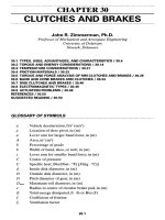
An
example
of
results obtained
from
a
widely used production inspection
method
is
shown
in
Fig. 40.15
([40.5]).
Line
1 was
obtained
from
some accurate data
from

a
table
of 6
values
and the
corresponding
s(0)
values. Next,
two
boundary
curves were obtained
from
the
basis curve
by
adding
and
subtracting
10
percent.
This
was an
arbitrary decision,
it
being assumed
that
any
acceleration curve con-
tained between such boundaries would
be

satisfactory.
These
are
shown
as
upper
and
lower bounds
in
Fig. 40.15.
The
main drawback
of the
method
is
that only maxi-
mum
values
of
actual acceleration diagrams have been taken into account.
It is
important
to
realize that waviness
of the
real
acceleration curve
may
cause more
vibration troubles than will single local surpassing

of
boundary curves.
A
much better method
is
that
of
measuring
the
real acceleration
of the
follower
in an
actual
cam
mechanism
at the
operating
speed
of the cam by
means
of
high-
quality
accelerometers
and
electronic equipment.
To
illustrate
the

importance
of
proper
measurements
of the cam
profile,
we
show
the
results
of an
investigation
of
FIGURE
40.15 Example
of
inspection technique based
on
acceleration diagram
obtained
from
accurate static measurements
of the cam of the
Henschel
internal com-
bustion engine.
the
mechanism used
in the
Fiat

126
engine
([40.6]).
Those
results
are
shown
in
Figs.
40.16
and
40.17.
The
acceleration diagram
of
Fig.
40.160
was
obtained
from
designer
data
by
using
Eq.
(40.29).
The
diagram plotted
as a
broken line

(1) in
Fig.
40.166
comes
from
accurate measurements
of a new
profile.
Here
again
Eq.
(40.29)
was
applied.
The
same profile
was
measured again
after
1500 hours
(h) of
operation,
and
the
acceleration diagram
is
plotted
by a
solid line
(2) in

Fig.
40.166.
Comparing
curves
1 and 2 of
Fig.
40.166,
we can see
that
the
wear
of the cam
smoothed some-
what
the
waviness
of the
negative part
of the
diagram. Accelerations
of the
follower
induced
by the
same
new cam in the
actual mechanism (Fig. 40.16c) were measured
as
well
by

electronic equipment
at the
design
speed,
and
results
of
that
experiment
are
presented
in
Fig.
40.16d
and
e.
It is
obvious
from
comparison
of the
diagrams
in
Fig. 40.166
and d
that
the
response
of the
system

differs
to a
considerable extent
from
the
actual input.
FIGURE
40.16 Comparison between results obtained
from
static measurements
of the
Fiat
126
cam
profile
[(a)
and
(b)]
and
acceleration curves obtained
at
design speed
on the
actual engine
[(d)
and
(e)].
Diagram
d was
obtained

for a
zero value
of
backlash
and
diagram
e for the
factory-
recommended
0.2-mm
backlash.
FIGURE
40.17 Changes
of
acceleration diagram caused
by the
wear
of the cam
profile
of
the
Fiat 126.
Eight
new
cams
of the
same engine were later used
in two
separate laboratory
stands

to
find
the
influence
of
cam-surface wear
on
dynamic properties
of the cam
system. Some
of the
obtained results
are
presented
in
Fig. 40.17.
We can
observe
there that some smoothing
of the
negative part
of the
curve (registered
as
well
by
statistical measurements) took place after 1500
h.The
general character
of the

accel-
eration curve remained unchanged, however. (That observation
was
confirmed
later
by
a
Fourier analysis
of all the
acceleration signals.)
The
conclusion derived from
that
single experiment
is
that dynamic imperfections
of the cam
system introduced
by
the
process
of cam
manufacturing
may
last
to the end of the cam
life.
40.3.1
Finite-Difference Method
Geometric acceleration

of the
follower
s"
may be
estimated
by
using accurate values
of
its
displacement
s
from
a
table
of 6
versus
s(0),
which comes
from
the
designer's
calculations
and/or
from
accurate measurements
of the
actual
cam
profile. Denoting
as 5/ _

i,
5/, and s/
+
i
three
adjacent
values
of s in
such
a
table,
and
designating their
second
finite
difference
as
A/',
we
have
c?
=
1
A"-
fr-i-2fr + fr +
i
(4028^
Sl
~
(AG)

2
A
'
"
(A6)
2
(4U
'
Z8)
where
A0 =
constant increment
of the
cam's angular displacement
6. A
more
accu-
rate value
of
S?
can be
found
from
the
average weighted value
(Oderfeld
[40.3])
by
using
entries

of 11
adjacent
A"
from
the
table
of s
versus
5(6):
«=
-&?'£*#+>
(
40
-
29
>
The
weights
W
7
are
given
in
Table
40.5.
TABLE
40.5
Weights
Used
in the

Improved
Finite-
Difference
Method
j
O ±1 2 ±3 ±4 ±5
Wj
0.31 0.25 0.13 0.015
-0.025
-0.025
An
example
of an
acceleration diagram
/'(0)
of a
certain
cam
obtained using
the
finite-difference
method
is
presented
in
Fig.
40.18.
40.4
FORCEANDTORQUEANALYSIS
A

typical approach
to
dynamic analysis
of a
rigid
cam
system
can be
illustrated
by an
example
of a
mechanism with
a
reciprocating roller
follower.*
A
schematic drawing
of
such
a
mechanism
is
depicted
in
Fig.
40.19«.
For the
upward motion
of the

fol-
1
Suggestion
of
Professor Charles
R.
Mischke, Iowa State University.
FIGURE 40.18
Acceleration
diagrams
obtained
in the
static way. Curve
1 is
from
Eq.
(40.28),
curve
2
from
Eq.
(40.29).
lower,
we
assume that
the
follower's stem
4
contacts
its

guideway
at
points
B and C.
As a
result
of its
upward motion,
the
Coulomb friction
at B and C is
fully
developed
and tan
\|/
=
fi.The
free-body diagram
of
links
3 and 4 is
shown
in
Fig.
40.19&
The cam
force
F
23
can be

resolved into
two
components:
P
CT
in the
critical-angle
(y
cr
)
direction
to
sustain motion against
friction,
and
P
y
in the y
direction
to
produce accelerated
motion
or to
oppose other forces.
It can be
found
from
the
geometry
of the

follower
that
Tcr
=
|-tan-',(^-f
-l)
(40.30)
where
a
=
I
8
-R
0
-
R
r
.
For y >
y
cr
,
the
cam-follower system
is
self-locking,
and
motion
is
impossible. From

the
force triangle
in
Fig.
40.195
and the
rule
of
sines,
FIGURE
40.19
Force
analysis
of
reciprocating
roller-follower
cam
system.
sir^^
smy
cr
After
finding
the
vertical component
P
y
for
constant
CO

2
I
from
the
force-equilibrium
equation, substituting into
Eq.
(40.31),
and
solving
for
F
23
,
we
have
p
_ sin
y^mco^"+
fa+
PQ
(4032)
23
sin(y
cr
-y)
where
m
=
mass

of
follower
k =
spring rate
of
retaining spring
p;=p
4
+fc8
5 =
preset
of
spring
fc8
=
P
0
;
this
force
is
called preload
of
spring
For
F
23
=
O,
roller

and cam
lose
their contact.
The
result
is
called jump
([40.7],
[40.8]).
Assuming
F
23
=
O,
we can
find
the
jump speed
of the cam
from
Eq.
(40.31).
The
jump
occurs
for the
upward movement
of the
follower
at

«**
V^
(40.33)
Since
s is
always positive, jump
may
occur only
for
negative values
of
s".
To
prevent
jump,
we
increase preload
P
0
or the
spring
rate
or
both.
The
driving torque
is
T
12
=

Sm
J
cr
Sm
I
(R
0
+
R
r
+
sXmcoiiS"
+ ks +
P'*)
(40.34)
sin
(y
cr
-
y)
We
recall that according
to Eq.
(40.25),
y
-
tan-
1
(40.35)
'

s
+
R
0
+
R
r
v
'
When motion
is
downward,
the
contact point
of
mating surfaces goes
to the
right
side
of the
roller,
cam
force
F
23
changes inclination,
and new
contact points
D and E
in

the
follower's guideway replace
old
ones
(B and C,
respectively).
The new
point
of
concurrency
is now at
F'.
Since
in
most practical cases points
F and
F'
almost
coincide,
we can
assume that both
the
point
of
concurrency
and the
line
of
action
of

force
P
cr
are
unchanged.
A new
vector
P
CT
(broken line)
is
rotated
by
180° with
respect
to the old
one.
It is
easy
to see in
Fig.
40.19/?
that
F
23
for
downward motion,
when
y and
P

y
equal those
for the
upward motion,
is
always smaller than
F
23
for
upward
motion.
40.4.1
Springs
In
cam-follower systems,
the
follower must contact
the cam at all
times. This
is
accomplished
by a
positive drive
or a
retaining spring. Spring forces should always
prevent
the
previously described jump
of the
follower

for all the
operating speeds
of
the
cam. Thus
the
necessary preload
P
0
of the
spring
and its
spring
rate
k
should
be
chosen
for the
highest possible velocity
of the
cam.
By
plotting inertial
and
spring
forces,
we can
find
values

of
preload
P
0
and
spring
rate
k
that will ensure
sufficient
load margin
for the
total range
of the
follower displacement.
We use
here
only
the
negative
portion
of the
acceleration curve. Since
the
follower
must
be
held
in
contact

with
the
cam, even while operating
the
system with temporary absence
of
applied
forces,
that part
of the
cam-system synthesis
may be
accomplished without applied
forces.
At the
critical location, where both curves
are in
closest proximity,
the
spring
force
should exceed
the
inertial force with friction
corrections
included
by not
less
than
25 to 50

percent.
40.5
CONTACTSTRESSANDWEAR:
PROGRAMMING
Let us
consider
the
general case
of two
cylinderlike surfaces
in
contact. They
are
rep-
resented
by a cam and a
follower.
The
radius
of
curvature
of the
follower
P
1
is
equal
to the
radius
of the

roller
R
r
for the
roller follower,
and it
goes
to
infinity
for a flat