House price model based on maginal analysis of house market
Bạn đang xem bản rút gọn của tài liệu. Xem và tải ngay bản đầy đủ của tài liệu tại đây (635.19 KB, 24 trang )
House Price Model Based on Marginal Analysis of House
Market
(Hay Nong Tsinghua University; Asian Economics Theory Research Center)
The paper built the basic theoretical model for urban house price, based on a
marginal analysis of house market. The contributions are the three. (1) We discovered,
in real world’s house market, there are three factors that strongly influence house price,
and we show the reason. (2) We built a three factors house price model, and tested the
model by empirical data. The model explains real world’s house price better than
present models. (3) The new model is the more general model, present house price
models, such as hedonic house price model, are the special situation of the new model.
1. Introduction
The value of house constitutes the major part of wealth. Such as, in China, the
value of house constitutes three quarters of total household wealth, and, in the United
States, the value of house constitutes one third of total household wealth (CGB, et al,
2018). Then, how house’s value or price is decided, is important both in theory and in
practice. But, till now, a basic theoretical model for urban house price is still needed.
Hedonic house price model is widely used by researchers to explain house price,
such as Kain and Quigley (1970), Wabe (1971), Evans (1973), Paul Cheshire, et al
(1995), Wen Hai-zhen (2005). Hedonic house price model argues house price is decided
by house’s objective attributes or characteristics, such as house’s size, house’s distance
to city center, etc. We use z ( z1 , z2 ,...., zn ) to represent one house’s attributes, then,
hedonic house price model is p f ( z ) f ( z1 , z2 ,...., zn ) .
Hedonic house price model only considers one house’s own attribute in price
decision, but as shown in Section 6, in real world’s house market, house attribute on
city periphery and house production cost on city periphery also strongly influence
house price (see Figure 1, Figure 2 in Section 6).
Why attribute and production cost of house on city periphery have strong influence
on house price? The reason can be found by marginal analysis of house market. In house
1
Electronic copy available at: />
market of one city, when an extra unit of house is built, the extra unit of house will often
be built on city periphery (see §3). As known by economists, the extra unit of
commodity has strong influence on market price (Ricardo 1817, Marshall 1890,
Samuelson 2005, etc.). Such as, Samuelson (2005), Mankiw (2016) etc. argued, in
perfectively competitive market reached long run competitive equilibrium, the cost of
extra unit of commodity (the marginal cost) decides commodity’s market price. And,
it’s obvious that, when attribute is considered in price decision, the attribute of the extra
unit of commodity also will influence commodity’s market price. Such as, as the newly
produced computer (the extra unit of computer provided to market) has better attribute
such as higher CPU speed, the old computer’s price will often drop down.
Then, totally, when attribute is considered in house price decision, in the city, there
are three factors that strongly influence house price. The three factors are house’s own
attribute, house attribute on city periphery (the extra unit house’s attribute), house
production cost on city periphery (the extra unit house’s production cost). Hedonic price
model only considers one factor and ignores the other two, then has obvious limitations.
Traditional economics assumes commodity is homogeneous, and argues, at long
run competitive equilibrium, commodity’s price equals the long run marginal cost
( Mc0 ) (see literature review in §2). In house market, the extra unit of house produced
is often on city periphery, then, house’s marginal cost ( Mc0 ) is just the production cost
of house on city periphery ( c0 ), then, traditional economics’ house price model will be
p Mc0 c0 (§2). Traditional economics’ house price model didn’t consider house
attribute, but in house market, house attribute does strongly influence house price.
We aim to build a basic theoretical model, then, we set some assumptions, and
assume house market is perfectively competitive and reached long run equilibirum. We
found, in perfectively competitive market reached long run equilibrium, under certain
assumptions such as houses have a homogeneous attribute, quality, house price will be
(1)
p
q
q( z )
c0
c0
q0
q ( z0 )
where p is one house’s price, q q( z ) is this house’s quality, q0 q ( z0 ) is the
2
Electronic copy available at: />
quality of house on city periphery, c0 is the production cost of the house on city
periphery. Here, house’s quality is a function of house’s attributes. z ( z1 , z2 ,...., zn )
are one house’s own attributes, z0 z10 , z20 ,...., zn0 are attributes of house on city
periphery. The deduction of formula (1) is arranged in Section 3.
Formula (1) looks new, but, the key logic of formula (1) is quite simple, price
equals marginal cost, one basic idea of present economics. Formula (1) can be changed
into
p c0
. Here, p pq is the price of house quality, c0 Mc0 Mcq is the
q q0
q0 Mq0
q
marginal cost to provide house qualtiy (see §4). Then, formula (1) becomes
pq Mcq
The above equation means, price of house quality pq equals marginal cost of house
quality Mcq . That price equals marginal cost is one basic idea of present economics
(see Samuelson et. al. 2005, Varian 2014, Mankiw 2016). This means, formula (1) is
only a use of present economics, but at quality or attribute level.
We tested formula (1) by empirical data, and found, formula (1) does exist in real
world’s market. In the test, the significance is lower than 0.01.
Formula (1) considers all the three factors ( z , z0 , c0 ) in house price decision.
Hedonic house price model only considers house’ own attribute z , and ignores z0 , c0 .
Traditional economics’ house price model only considers cost c0 , and ignored z , z0 .
Then, formula (1) has obvious advantages. We find, formula (1) explains real world’s
house price better than other two models. (see §6, 7).
By data of 31 major cities in China, we provided a comparison of the three models
in explaining real world’s house price (§6.3). The result of comparison is in table below.
Model Name
q( z )
c0
q ( z0 )
This paper’s house price
model, formula (1)
p
Traditional economics’
house price model
p Mc0 c0
p f ( z)
Hedonic house price model
Explaining
Variable
Model Form
Estimated Model
R-square
e0.043d
c0
e0.043d0
0.754
c0
p c0
0.453
z
p e3.1680.014d
0.019
z , z0 , c0
p
3
Electronic copy available at: />
In the comparison, we use per square meter house price (p), and we use house’s
distance to city center (d) to represent house’s attribute, since in major cities of China,
house’s distance to city center is the most important attribute that influences per square
meter house price. (see §6.3).
From the comparison, we find, formula (1) has the highest R-square. This means,
formula (1) explains real world’s house price better than other models. Here, the Rsquare of formula (1), 0.754, is high enough, since we only consider one attribute
(distance to city center d) of house, and house has several attributes that influence price.
Here, hedonic price model’s R-square is the lowest, only 0.019. The reason is, as
analyzed in §5, hedonic house price model fits to explain house price in the same city,
but here, the house price is from 31 cities, not from the same city.
We find, hedonic house price model can be seen as the special situation of formula
(1) when c0 , z0 are given. When c0 , z0 are given, c0 and q0 q ( z0 ) are given,
let
c0
k , formula (1) becomes p q c0 c0 q k gq( z1 , z2 ,..., zn ) f ( z1 , z2 ,..., zn ) ,
q0
q0
q0
here, f ( z1 , z2 ,..., zn ) is also a hedonic house price model (see §6). And, traditional
economics’ house price model is also the special situation of formula (1), when houses
are homogeneous in attribute. When houses are homogeneous in attribute, z z0 , then,
q q( z ) q( z0 ) q0 , then formula (1) becomes p 1gc0 c0 .
This paper’s contributions are the following three. (1) We discovered, in real
world’s house market, there are three factors that strongly influence house price, and
we show the reason. (2) We built a three factors house price model, and tested the model
by empirical data. The model explains real world’s house price better than present
models. (3) The new model is the more general model, while present house price models,
such as hedonic house price model, are the special situation of the new model.
The remainder of the paper is organized as follows. Section 2 provides literature
review. Section 3 provides a marginal analysis of house market, and builds the model.
Section 4 provides the more theoretical expression of the model. Section 5 shows the
model’s difference from hedonic house price model. Section 6 tests the model. Section
7 explains real world’s house price by the model. Section 8 concludes.
4
Electronic copy available at: />
2. Literature Review
Traditional economics assumes commodity is homogeneous, and argues, at long
run competitive equilibrium, price equals the minimum long run average cost
and equals long run marginal cost ( Mc0 ), which means p LACmin Mc0 , such as
Samuelson et. al. (2005, 2010), Pindyck et. al. (2013), Varian (2014), Mankiw (2016).
And, the idea that price equals marginal cost can also be traced back to David
Ricardo(1817), Stuart Mill (1848), Alfred Marshall (1890), etc., even Karl Marx (1867).
The assumption, commodity is homogeneous, implies that commodity is the same
in attribute, such as each computer has the same CPU speed. By assuming commodity
is homogeneous, traditional economics excludes attribute and only considers cost in
price decision. But in real world’s market, commodity is often heterogeneous in
attribute and attribute does strongly influence price. Such as, in real world’s computer
market, computer may have different CPU speeds, and the computer with higher CPU
speed will often have higher price. Then, to explain real world’s price, attribute should
be considered.
In big cities, when house is built in the city, mostly, the land near city center is
better land and will be used first, after the land near city center is used up, the land farer
from city center will be used. Then, in big city, when an extra unit of house is built, the
extra unit of house will be built on city periphery. In traditional economics, marginal
cost is defined as the total cost increased when an extra unit of commodity is produced.
Then, according to the definition of marginal cost, in house market, the marginal cost
of house ( Mc0 ) will be the production cost of house on city periphery ( c0 ). Then,
traditional economics’ house price model will be p Mc0 c0 .
It’s obvious that, traditional economics’ house price model (house price equals
house’s marginal cost) cannot well explain house price in real world’s market. In real
world’s competitive house market, in big cities, house price on city periphery might
equal house’s marginal cost (house’s production cost on city periphery).1 But, house
As analyzed in section 3, on city periphery, there are often plenty of land to build house, then, the
supply of house is easily to be increased. Then, in competitive house market, on city periphery, if house
price is higher than production cost, more houses will be built, until house price equals production cost.
1
5
Electronic copy available at: />
price in city center will often be much higher than house’s marginal cost (house’s
production cost on city periphery). This means, house price in city center can’t be
explained only by house’s marginal cost.
Hedonic price model is widely used by researchers to explain house price, such as
Kain and Quigley (1970), Wabe (1971), Evans (1973), Paul Cheshire, et al (1995), Wen
Hai-zhen (2005). Hedonic house price model argues house’s price will be decided by
house’s attributes. The limitation of hedonic house price model is that, hedonic house
price model only considers house’s own attribute, but as shown in Section 6 (Figure 1,
2), attribute of house on city periphery and production cost of house on city periphery
also strongly influence house price. Then, hedonic price model in fact ignored the other
two important factors in house price decision, then, hedonic price model has obvious
limitations and cannot be the basic theoretical model for urban house price.
Besides above two major schools of house price model, some other house price
models were also built, such as James M. Poterba, et. al. (1991), Steven C. Bourassa et.
al. (2001), Peter Abelson et al (2005), etc. But these models also cannot theoretically
explain real world’s house price decision.
Till now, we still need a basic theoretical model for urban house price.
Olsen (1969) argued, in house market, different house has a homogeneous attribute,
house’s quality or house’s housing service, and, at long run competitive equilibrium,
houses will have the same quality/price.
Olsen (1969)’s idea is a good abstraction of the real world’s house price
phenomenon that better house has higher price. Such as, in real world’s house market,
in big cities, the house nearer to city center is often the better house (the house with
better transportation, shorter distance to office, better medical service, etc.), and, the
house nearer to city center often has higher per square meter house price.
That better commodity (commodity with better attribute or higher quality) has
higher price is also widely existing in many other markets. Such as, in iron ore market,
Then, on city periphery, house’s tends to equal house’s production cost . While as analyzed in the
following, house’s production cost on city periphery represents house’s marginal cost. Then, house
price on city peripehry tends to equal house’s marginal cost.
6
Electronic copy available at: />
the iron ore that contains more iron element often has higher price.
This paper assumes better house has higher price, then, Olsen (1969)’s idea will
be used in this paper, because Olsen (1969)’s idea is a good abstraction of the price
phenomenon that better house has higher price.
3. A Marginal Analysis of House Market, and House Price Model
Since we aim to build a basic theoretical model, then, in this paper, we always
assume house market is perfectively competitive and reached long run competitive
equilibrium. We always assume house’s attribute is positive.
3.1 A Marginal Analysis of House Market
Marginal analysis can be widely used to explain consumer choice, producer choice
and price decision. Marginal analysis was used by many economists, such as Menger
(1871), Jevons (1871), Walras (1899), Ricardo (1817), Mill (1848), Marshall (1890),
Clark (1899), etc. Here, we provide a marginal analysis of house market. In this
marginal analysis, house attribute is considered.
As already mentioned, in big cities, when house is built in the city, mostly, the land
near city center is better land and will be used first, after the land near city center is
used up, the land farer from city center will be used. Then, in big city, when an extra
unit of house is built, the extra unit of house will be built on city periphery.
The Production Cost and the Attribute of the Extra Unit of House
House is the commodity that has several attributes, such as house’s distance to city
center, house’s size, etc. House’s these attributes can be divided into two categories.
The first category of attributes are attributes that are directly decided by house’s
location, such as house distance to city center, etc. The second category of attributes are
attributes of house itself, such as house’s size, house’s decoration, etc. The second
category of attributes are not directly decided by house’s location, and are often called
structural attributes.
In this paper, one house’s all attributes are represented by
z ( z1 , z2 ,...., zn )
Where z is the vector of house attributes, z1 , z2 ,...., zn are one house’s all attributes.
7
Electronic copy available at: />
In this paper, for simplification, we assume houses are the same in the second
category of attributes. This also means, we assume houses are the same except houses
are on different locations. Under this assumption, in the same city, once the location of
house is given, house’s attributes z ( z1 , z2 ,...., zn ) are given.
As mentioned above, in house market, when an extra unit of house is built, the
extra unit of house will be built on city periphery. We use z0 z10 , z20 ,...., zn0 to
represent the attributes of house on city periphery. Then, above on above analysis we
can find, in house market, when an extra unit of house is built, the extra unit of
house will have attributes z0 z10 , z20 ,...., zn0 . In one city, at given time, the city
periphery will be on given location or given place, then, z0 z10 , z20 ,...., zn0 are given.
As mentioned above, in house market, when an extra unit of house is built, the
extra unit of house will be built on city periphery. We use c0 to represent the
production cost of house on city periphery. Then, when an extra unit of house is
produced, the production cost of the extra unit of house will be c0 .
Then, above marginal analysis shows, in house market of one city, when an extra
unit of house is built, the production cost of the extra unit of house is c0 , the attributes
of the extra unit of house are z0 z10 , z20 ,...., zn0 .
The Three Factors that Influence House Price
Traditional economics argues, the production cost of extra unit of commodity (the
marginal cost) will influence commodity’s price (Samuelson 2005, Mankiw 2016, etc.).
This argument was verified by empirical data of real world’s house market. As shown
by figure 2 in Section 6, in 31 major cities of China, as the the production cost of house
on city periphery (the production cost of extra unit of house) goes up, house price in
the city often goes up.
Here, a new question arises. Will the attribute of extra unit of commodity also
influence commodity’s market price?
If we observe the real world’s prices, we can find, the answer is yes. Such as, in
computer market, the newly produced computers can be seen as the extra units of
computer provided to the market. And, in real world’s computer market, as the newly
8
Electronic copy available at: />
produced computer has better attribute, such as higher CPU speed, the old computer’s
price will often drop down.
This paper found, in house market, the attribute of the extra unit of house strongly
influence house price. As illustrated by figure 1 in section 6, in 31 major cities of China,
house price is strongly influenced by the attribute of house on city periphery, while the
attribute of house on city periphery represents the attribute of extra unit of house.
As mentioned above, the attribute of house on city periphery (the attribute of the
extra unit of house) influences house price, the production cost of house on city
periphery (the production cost of the extra unit of house) influences house price. And,
it’s obvious that, one house’s own attributes will influence this house’s price. Then,
totally, there are three factors that influence one house’s price. The three factors are:
one house’s own attribute z , the attribute of house on city periphery z0 , the
production cost of house on city periphery c0 .
Since in house market, there are three factors that influence house price, then,
house price model should consider all the three factors in house price decision. In the
following, we will discover how house price is decided by the three factors.
The Price and the Attribute of the Extra Unit of House
Marginal cost is the total cost increased when an extra unit of commodity is
produced. Then, according to the definition of marginal cost, in house market, the
marginal cost ( Mc ) will be the production cost of house on city periphery ( c0 ), then
Mc c0
Marginal revenue is the total revenue increased when an extra unit of commodity
is produced. And as mentioned above, in house market, the extra unit of house will be
on city periphery. Since house market is assumed to be perfectively competitive, then,
according to the definition of marginal revenue, in house market, the marginal revenue
( Mr ) will equal the price of house on city periphery ( p0 ). then
Mr p0
According to traditional economics, in perfectively competitive market reached
long run competitive equilibrium, marginal revenue ( Mr ) will equal marginal cost
9
Electronic copy available at: />
( Mc ), then we get
p0 Mr Mc c0
This means, house price on city periphery ( p0 ) will equal the production cost of
house on city periphery ( c0 ).
p0 c0
It’s easy to understand why on city periphery house price will equal house
production cost. On city periphery, since there are often plenty of land to build house,
then, the supply of house on city periphery is easily increased. If the price of house on
city periphery is higher than production cost, there will exist profit, then, more houses
will be built, then house price will drop down, until price of house equals production
cost of house.
The above marginal analysis shows, in perfectively competitive house market
reached long run competitive equilibrium, the price of house on city periphery will be
p0 c0 . Since as set in above, the attributes of house on city periphery is
z0 z10 , z20 ,...., zn0 . Then, we can find, in perfectively competitive house market
reached long run competitive equilibrium, the price of house on city periphery will be
p0 c0 , the attributes of house on city periphery is z0 z10 , z20 ,...., zn0 . Note that, in a
given city, at given time, c0 and z0 are given (see footnote in page 12).
As analyzed, the house on city periphery represents the extra unit of house in house
market. Then, the above analysis also means, in perfectively competitive house market
reached long run competitive equilibrium, when extra unit of house is built, the extra
unit of house will have a price p0 c0 , and, the extra unit of house have attribute
z0 z10 , z20 ,...., zn0 .
3.2 The Price Model When House Has One Cardinal Attribute
Traditional economics argues, in perfectively competitive market at long run
competitive equilibrium, commodity’s price is decided by the production cost of extra
unit of commodity (Samuelson 2005, Mankiw 2016, etc., even Marshall 1890).
Traditional economics’ this argument was based on the assumption that
commodity is homogeneous, such as each unit of computer is homogeneous. But, in
10
Electronic copy available at: />
house market, houses are heterogeneous in attribute, and house attribute does influence
house price. We argue, in house market, for one house with given attribute, this house’s
price is decided by both the production cost of the extra unit of house and the
attribute of the extra unit of house.
As analyzed above, in perfectively competitive house market reached long run
competitive equilibrium, when extra unit of house is built, the extra unit of house will
have a price p0 c0 , and, the extra unit of house have attribute z0 z10 , z20 ,...., zn0 .
And, c0 , z0 are given.
Suppose in the city, house A’s attributes are z ( z1 , z2 ,...., zn ) , z z0 . This
means, house A has better attributes than the extra unit of house (the house produced
on city periphery). It’s easy for us to know that, house A’s price p A will be higher than
p0 c0 , since house A has better attributes. Why house A will have a higher price? The
reason lies in consumer’s choice behavior. Here, if house A’s price is the same as or
even lower than the extra unit of house’s price, all consumer will choose house A, then,
the house A’s price will go up (The price of the extra unit of house is assumed given).
But the above analysis only tells us whether house A’s price is higher or lower
than p0 c0 , since the above analysis is only qualitative. The important question is,
quantitatively, how house A’s price is decided?
To answer this question, a deep analysis on consumer choice is required, which
might need 20 pages. Fortunately, Olsen (1969)’s idea can help us to answer this
question quickly.
Olsen (1969) argued, in house market, different house has a homogeneous attribute,
house’s quality or house’s housing service, and, at long run competitive equilibrium,
houses will have the same quality/price. Olsen (1969)’s idea is a good abstraction of
consumer’s influence on house price, better house (house with better attributes) will
have higher price.
Similar to Olsen (1969)’s idea, we assume each house has a homogeneous and
cardinal attribute, quality q . And, house’s quality q is function of house’s attributes.
Then
11
Electronic copy available at: />
q q( z ) q( z1 , z2 ,,..., zn )
where q is one house’s quality, z z1 , z2 ,,..., zn are this house’s all attributes.
As analyzed above, in perfectively competitive house market reached long run
competitive equilibrium, the extra unit of house will have attributes z0 z10 , z20 ,...., zn0
and price p0 c0 . The house with attributes z0 z10 , z20 ,...., zn0 will have a quality
q0 q( z0 ) q( z10 , z20 ,...., zn0 ) . Then, in perfectively competitive house market reached
long run competitive equilibrium, the extra unit of house will have quality
q0 q( z10 , z20 ,...., zn0 ) and price p0 c0 .
Suppose there is one house in the same city, its attributes are z z1 , z2 ,,..., zn and
quality is q q( z1 , z2 ,,..., zn ) , and this hosue’s price is p . Similar to Olsen(1969)’s
idea, we assume that, in perfective competitive market reached long run competitive
equilibrium, houses will have the same quality/price, then, we can get
q q0 q0
= ,
p p0 c0
then we get
p
(1)
q
q( z )
c0
c0
q0
q ( z0 )
where p is one house’s price, q is this house’s quality, q0 is the quality of extra
unit of house and q0 is also the quality of house on city periphery, c0 is the
production cost of the extra unit of hosue and c0 is also the production cost of house
on city periphery. Here, the house market is assumed to be perfectively competitive and
reached long run equilibrium. In a given city, at given time, z0 , q0 , c0 can be seen as
given.1
This paper assumes house’s attribute is decided by house’s location. In a given city at given time, the
city periphery will be on given location, then, house’s attributes are given, then, the quality of house is
given. In a given city at given time, the production cost is also given.
If we give up that assumption that house’s attributes are decided by location, in given city at given
1
time,
z0 , q0 , c0
are also given. In a given city, at given time, when house market reached long run
competitive equilibrium, house produced on city periphery will have the best match of house attributes
and production cost under given technology and factor prices (labor cost, land cost etc.). Here, the best
match of house attributes and production cost can be seen as the solution of the optimum problem of
house production, then can be seen as given, though attributes of house and production cost of house
might be related. And, house’s attributes are given means house quality is given. For more analysis,
please contact the author.
12
Electronic copy available at: />
After a test in §6 and analysis in §7, we will find, formula (1) does exist in real
world’s house market, and can explain real world’s house price better than other
models, such as hedonic house price model.
Totally, formula (1) considers three factors in house price decision, the three
factors are: one house’s own attributes ( z ), attributes of house on city periphery ( z0 ),
and production cost of house on city periphery ( c0 ). Formula (1) represents this paper’s
three factors house price model.
3.3 The Price Model When House Has One Ordinal Attribute
Formula (1) is the theoretical model for house price when house has one cardinal
attribute, house’s quality. We created the concept of house quality, to discover the basic
law of house price decision. We do find the basic law of house price decision, which is
formula (1). But, in real world’s market, house’s attribute is often ordinal, not cardinal,
such as, house’s distance to city center is only an ordinal attribute.
Formula (1) can help us to understand the house price decision when house has
one ordinal attribute. Based on formula (1), we can find, when house has one ordinal
attribute, there will exist the following three qualitative relationships in house market.
Relationship 1 Given production cost of house on city peripehry ( c0 ) and the
attribute of house on city periphery ( z0 ), house price ( p )will be positively related with
house’s attribute ( z ).
Relationship 2 Given house’s attribute ( z ) and the production cost of house on
city peripehry ( c0 ), house price ( p )will be negatively related with the attribute of house
on city periphery ( z0 ).
Relationship 3 Given house’s attribute ( z ) and the attribute of house on city
periphery ( z0 ), house price ( p ) will be positively related with production cost of house
on city periphery ( c0 ).
The above three relationships represents this paper’s house price model when
house has one ordinal attribute.
We argue, when house has several ordinal attributes, the basic law of house price
13
Electronic copy available at: />
decision will be similar to house price decision when house has one ordinal attribute.
In real world’s house market, house’s attribute is often ordinal, then, the above three
relaitonships can be more frequently used to explain real world’s house price.
4. A More Theoretical Expression of the House Price Model
As already mentioned, in perfectively competitive house market reached long run
competitive equilibrium, house’s marginal cost ( Mc0 ) will be the production cost of
house on city periphery ( c0 ), then, Mc0 c0 . In this paper, the quality of the extra unit
of house is called marginal quality. In house market, house’s marginal quality ( Mq0 )
will be the quality of house on city periphery ( q0 ) , then, Mq0 q0 . Since Mc0 c0
and Mq0 q0 , then formula (1) can also be expressed by the following model
p
(2)
q
Mc0
Mq0
where Mq0 is house’s marginal quality at equilibirum, Mc0 is house’s marginal cost
at equilibrium. Formula (2) is a more theoretical expression of this paper’s house price
model.
Further analysis shows, formula (2) is also a general price model for various
commodities in competitive market, when commodity’s quality or attribute is
considered in price decision.1 This means, this paper’s house price model is not an
isolated model, but a special use of a more general model in house market.
We asssume house and house’s quaity are dividable and additive. We set that, H
is the quantity of house added, c is the production cost added because of H , q
is the house quality added because of H . As analyzed in above, c0 Mc0 =
the marginal cost to produce house, q0 Mq0
1
q
H
is the marginal quality in
The proving of (2) is similar to the proving of formula (1). The only difference is, here,
Mq0 , Mc0
c
is
H
p, q,
are price, quality, marginal quality, marginal cost of commodity. The two conditions for
us to get formula (2) are: (a) commodities have the same quality/price, (b) marginal revenue equals
marginal cost. More analysis is in the author’s working paper “A two factors price model based on
deeper research of consumer choice”.
14
Electronic copy available at: />
producing house. Then
c0 Mc0 c / H c
c
Mcq . This means, 0 =Mcq in
q0 Mq0 q / H q
q0
fact is the marginal cost to provide house quallity.
Formula (1) can be changed into
analyzed above ,
p c0 p
.
pq is the price of house quality. As
q q0 q
c0
=Mcq is the marginal cost to provide house quallity. Then,
q0
formula (1) becomes
pq Mcq
The above equation means, the price of house quality equals the marginal cost to
provide house quality. This means, the key logic of formula (1) is quite simple, at
quality or attribute level, price equals marginal cost. That price equals marginal cost
is one baisc idea of present economics’ price theory. This means, formula (1) is only a
use of present economics’ price theory, but at quality or attribute level.
Rosen (1969) already addressed pq Mcq , but Rosen didn’t develop a model like
formula (1) based on pq Mcq . As analyzed in this paper, formula (1) is the basic
theoretical model for urban house price, and well explains real world’s house prices.
5. The Difference from Hedonic House Price Model, etc.
We can find, this paper’s house price model, formula (1), considers all the three
factors that influence house price, then is the more general house price model. Hedonic
house price model and traditional economics’ house price model considers only one
factor, and can be seen as the special situation of formula (1).
Hedonic house price model argues house’s price will be decided by house’s
attributes. According to hedonic house price model, house price will be
p f ( z)
Where p is one house’s price, z z1 , z2 ,..., zn are this house’s attributes.
Hedonic house price model only considers z (one house’s own attributes) in this
house’s price decision. While this paper’s house price model, formula (1), considers
15
Electronic copy available at: />
z , z0 , c0 in house price decision.
After the following analysis, we can find, hedonic house price model is a special
situation of formula (1) when z0 (attribut of house on city periphery) and c0
(production cost of house on city periphery) are given.
In formula (1), q q( z1 , z2 ,..., zn ) , z1 , z2 ,..., zn are one house’s attributes. In formula
(1), when production cost of house on city periphery ( c0 ) and attribute of house on city
periphery ( z0 ) are given, c0 and q0 q ( z0 ) are given, let
c0
k , then k is also
q0
given. Then, formula (1) will become
p
c
q
c0 0 q k gq( z1 , z2 ,..., zn )
q0
q0
Let k gq( z1 , z2 ,..., zn ) f ( z1 , z2 ,..., zn ) . Then, formula (1) becomes
p f ( z1 , z2 ,..., zn )
The model is also a hedonic house price model.
The above analysis means, hedonic house price model is only a special situaiton
of this paper’s house price model. The special situation is that, attribute of house on
city periphery ( z0 ) and production cost of house on city periphery ( c0 ) are given.
When attribute and production cost of house on city periphery are given? The
answer is, in the same city at given time, attribute and production cost of house on city
periphery are given. Because, in different cities, the attribute of house on city periphery
and the production cost of house on city periphery will be different, and, in the same
city, as time elapses, the cost to produce house on city periphery and the attribute of
house on city periphery will change.(Note that, in the same city, in different year, city
peripehry might be at different place, since as time elapses city might become larger or
smaller.)
Then, according to formula (1), we can find, hedonic house price only fits to
explain the house price in the same city at given time, but cannot explain the house
price in many cities or the house price during many years.
16
Electronic copy available at: />
The empirical analysis in§6.3 shows that, hedonic house price model doesn’t fit to
explain the house prices in many cities, and, by evidence from real world’s market, we
can find that, hedonic house price model cannot explain house price during many years.
Such as, in Beijing City of China, during 2004-2020, the average house price went up
from 700 dollars per square meter to 8000 dollars per square meter, more than 10 times.
It’s obvious that, this rise of house price during 2004-2020 in Beijing cannot be mainly
explained by the rise of house’s attribute.
And, as analyzed by many researchers, hedonic house price model can explain
house price in the same city at given time.(see Kain and Quigley (1970), Wabe (1971),
Evans (1973), Paul Cheshire, et al (1995), Wen Hai-zhen (2005), etc.)
Formula (1) can explain house price in many cities and can explaing house price
during many years. Such as, the empirical analysis in§6.3 shows that, formula (1) can
explain house price in many cities. And, the analysis in §7 shows that, formula (1) can
explain house price during many years.
Traditional economics’ house price model will be p c0 (see §2). Traditional
economics’ house price model considers only one factor ( c0 ) and ignored the other two
( z , z0 ). Traditional economics’ house price model also can be seen as a special
suituation of this paper’s model, when houses are homogeneous in attribute. When
houses are homogeneous in attribute, then z z0 , then, q q( z ) q( z0 ) q0 , then,
formula (1) will become
p
q
c0 1gc0 c0
q0
which is just traditional economics’ house price model.
6. Test the Model
6.1 Test the House Price Model when House Has One Ordinal Attribute
Relationship 1,2,3 in §3.3 represents the house price model when house has one
ordinal attribute. Here, we will test Relationship 1,2,3, by data of 31 major cities in
China. The detailed test is arranged in Appendix A.1.
Since the three relationships are only qualitative, then, we will test the three
17
Electronic copy available at: />
relationships by figure and by correlation coefficient.
Relationship 2 is the new relationship discovered by this paper, then, we will focus
on Relationship 2. Relationship 2 shows that, one house’s price is negatively related
with the attribute of house on city periphery (given one house’s own attribute and given
the production cost of house on city peripehry).
In the test, house attribute is house’s distance to city center (d), house price is per
square meter price (In major cities of China, the distance to city center is the most
important attribute that influence per square meter house price).
After test, we find, the correlation coefficient between house price and
attribute of house on city periphery is -0.749, and the significance is less than 0.01.
This means, in real world’s house market, given house’s attribute and given production
cost of house on city periphery, house price is significantly negatively related with
attribute of house on city periphery.
Figure 1: House Price and Attribute of House on City Periphery
House Price
Attribute of House
on City Periphery
(Kilometers)
From the above Figure 1, we can find that, house price is obviously negatively
related with the attribute of house on city periphery (Here, one house’s own attribute
and the production cost of house on city periphery are given).
From the test, we also found that, given production cost and attribute of house on
city periphery, one house’s price is positively related with this house’s own attribute.
And, from the test, we also found that, given one house’s own attribute and given the
attribute of house on city periphery, one house’s price is positively related with the
production cost of house on city periphery. Figure 2 below shows that, house price is
obviously positively related with the production cost of house on city periphery.
18
Electronic copy available at: />
Figure 2: House Price and Production Cost of House on City Periphery
House Price
(1000/m2)
Production Cost
of House on
City Periphery
(1000/m2)
From the test, we find, the above Relationship 1, 2,3 in §3.3 do exist in real world’s
market. This also implies that, formula (1) is a successful theoretical model.
From the test, we find, in real world’s house market, house price in the city is
strongly influenced by each of the three factors: house’s own attribute, attribute of
house on city periphery, and production cost of house on city periphery.
6.2 Test the House Price Model when House Has One Cardinal Attribute
We tested formula (1) by 120 communities’ house price in 31 cities in china. After
hypothesis test, we find, formula (1) does exist in real world’s house market. The
detailed hypothesis test is in Appdendix A.2.
6.3 Comparision of the Three Different House Price Models
Base on above empirical data of 31 cities’ house market, we provide a comparison
of the three different house price models. For detail, see Appendix A.3.
Based on above data and formula (1), we got the following house price model. The
model represents this paper’s house price model.
(3)
p
q
q (d )
e 0.043d
c0
c0 0.043d0 c0
q0
q (d 0 )
e
0.043d
Where p is one house’s price, q e
is this house’s qualtiy, d is this house’s
0.043d0
distance to city center; q e
is qualtiy of house on city periphery, d 0 is city
periphery’s distance to city center. The R-square of the model is 0.754, which is high
enough, since here, we considers only one attribute of house in house price decision,
and house often has several important attributes that influence house price.
19
Electronic copy available at: />
Based on above data, we also got a hodenic house price model
p e3.1680.014d
the R-square of the model to explain house price is 0.019. Why the R-square of hedonic
house price model is quite low? The reason is, as analyzed in section 5, hedonic house
price model fits to explain house price in the same city at given time, but here, the data
of house price is from 31 cities, then, hedonic house price model loses its power.
As analyzed in §2, traditional economics’ house price model will be
p Mc0 c0
Where c0 is the production cost of house on city periphery. Based on above data of
house price, we find, the R-square of traditional economics’ house price model is 0.453.
As shown in the following table, we can find, formula (3) has the highest R-square
(0.754).This means, this paper’s house price model explains real world house price
better than other models. Here, the R-square (0.754) is high enough, since only one
attribute of house is considered in house price decision, while house has several
attributes that strongly influence house price.
Model Name
Model Form
Explaining
Variable
Estimated Model
R-square
z , z0 , c0
e0.043d
p 0.043d0 c0
e
0.754
q( z )
c0
q ( z0 )
This paper’s house price
model
p
Traditional economics’
house price model
p Mc0 c0
c0
p f ( z)
z
Hedonic house price
model
p c0
(Estimation is not needed)
0.453
p e3.1680.014d
0.019
7. Explaining Real World’s House Price
In this section, we can find, this paper’s house price model explains real world’s
house price much better than other models.
In real world’s house market, there are three important price phenomena. The three
price phenomena are very common, though some people might not notice them all.
The first phenomenon is that, in the same city, house on better location will has a
higher per square meter price. Such as, in big cities, the location nearer to city center is
20
Electronic copy available at: />
always the better location, and, in big cities, house nearer to city center always has a
higher per square meter price. Such as, as illustrated in the following Figure 3, in
Beijing City, house nearer to city center often has a higher per square meter price.
Figure 3: House Price and House Location (Beijing City)
House Price
(1000/m2)
180
160
140
120
100
80
60
40
20
0
Distance to
City Center
(Kilometers)
0 1 2 3 4 5 6 7 8 9 10 11 12 13 14 15 16 17 18
The second phenomenon is that, as the production cost of house goes up, house price
in the city will go up. Such as, in Beijing City, during 2004-2021, as the production cost
of house on city periphery went up from 300 dollars per square meter to 5000 dollars
per square meter, the average house price in the city went up from 700 dollars per square
meter to 8000 dollars per square meter.
The third phenomenon is that, as the city becomes larger, house price in city center
will become higher. Such as, as illustrated in the following figure 4, in 31 cities, the
larger city often has a higher city center house price. (Here, we use the distance between
city center and city periphery to represent city’s size, and, we use the relative house
price instead of house price to reduce the noise brought by house price level).
Figure 4: City Center House Price and City Size
City Center
House Price
6.00
5.00
4.00
3.00
2.00
1.00
0.00
0
10
20
30
40
Size of City
(Kilometers)
We argue, a successful house price model should be able to explain the above
three house price phenomena, since the above three house price phenomena are quite
21
Electronic copy available at: />
common in big cities around the world.
We can find, neither hedonic house price model nor traditional economics’ house
price model can explain all the above three important house price phenomena. Hedonic
house price model can explain the first houses price phenomenon (house on better
location has higher price), but cannot explain the second and the third house price
phenomenon. Traditional economics’ house price model can explain the second house
price phenomena (house price will go up as production cost goes up), but cannot explain
the first and the third house price phenomenon.
As mentioned in formula (1), this paper’s house price model is
p
q
c0
q0
where p is one house’s price, q is this house’s quality, q0 is the quality of house
on city periphery, c0 is the production cost of house on city periphery.
We can find that, this paper’s house price model can explain all the above three
house price phenomena.
The above house price model shows that, given q0 and c0 , one house’s price p
is positively related with this house’s quality q . And, according to the definition of
house quality in this paper, house on better location will have higher quality q . Then,
according to above house price model, in the same city at given time, house on better
location will have higher quality q , then will have a higher p ( As already analyzed,
in the same city at given time, q0 and c0 are given). Here, we can find that, this
paper’s house price model can explain the first house price phenomenon, house on
better location will have a higher price.
The above house price model shows that, given q and q0 , one house’s price p
is positively related with c0 (the production cost of house on city periphery),if the
production cost of house on city periphery ( c0 ) goes up, in the city, all house’s price
will go up. We can find that, this paper’s house price model can explain the second
house price phenomenon in real world’s market.
The above house price model shows that, given q and c0 , house’s price p is
22
Electronic copy available at: />
negatively related with q0 (quality of house on city periphery), if q0 goes down, p
will go up. When one city becomes larger and larger, compared with house in city center,
house on city periphery will have a relatively lower and lower quality ( q0 ).1 Then,
according to above house price model, (suppose the production cost of house on city
periphery c0 keeps unchanged), as the city becomes larger and larger, house price in
city center ( p ) will become higher and higher. We can find that, this paper’s house
price model can explain the third house price phenomenon, house price in city center
will become higher as city becomes larger.
The second house price phenomenon and the third house price phenomenon in fact
are the house price phenomenon during many years, since only during many years,
house’s production cost and city size might change dramatically. Then, the above
analysis in fact implies, this paper’s house price model can explain house price during
many years.
8. Conclusions
This paper developed a house price model, in perfectively competitive house
market reached long run competitive equilibrium. The house price model is
p=
q
c0
q0
where p is one house’s price, q is this house’s quality, q0 is the quality of house on
city periphery, c0 is the production cost of house on city periphery.
The house price model provides better explanation to real world’s house price than
other models, and can be the basic theoretical model for urban house price.
Reference
Adam Smith. (1776) 1976. An Inquiry into the Nature and Causes of the Wealth of Nations. Chicago:
The University of Chicago Press.
Alfred Marshall. 1890. Principles of Economics. London: Macmillan.
CGB (China Guangfa Bank), Southeast University of Finance and Economics. 2019. “2018 China
1
As the city becomes larger, compared with the house in city center, the house on city periphery will have
relatively worse and worse transportation, business environment, etc., since it becomes farer and farer away from
city center. This also means, as the city becomes larger, house quality on city periphery will become relative lower
and lower.
23
Electronic copy available at: />
Urban Household Wealth Health Report.” />David Ricardo. [1817]1976. On the Principles of Political Economy and Taxation. Beijing: The
Commercial Press.
Edgar O. Olsen. 1969. “A Competitive Theory of the Housing Market.” The American Economic
Review 59(4): 612-622.
Evans, A. W. 1973. The Economics of Residential Location. London: Macmillan.
Hal R. Varian.2014. Intermediate Microeconomics (9th Edition). New York, London: W. W. Norton &
Company.
James M. Poterba, David N. Weiland Robert Shiller. 1991. “House Price Dynamics: The Role of Tax
Policy and Demography,” Brookings Papers on Economic Activity, 1991(2):143-203.
John Bates Clark. (1908)1977. The distribution of wealth. A theory of wages, interest and profits.
London: MacMillan.
John Richard Hicks. 1939. Value and Capital. Oxford: Oxford University Press.
John Stuart Mill. [1848] 1991. Principles of Political Economy. Beijing: The Commercial Press.
Kahn, Barbara E.; Meyer, Robert J. 1991. “Consumer Multi-Attribute Judgments Under Attribute-Weight
Uncertainty.” Journal of Consumer Research 17(4): 508-522.
Kain, J. and J. M. Quigley. 1970. “Measuring the Value of Housing Quality.” Journal of the American
Statistical Association 65: 532-548.
Karl Marx. [1867]1975. The Capital. Beijing: The Commercial Press.
Kelvin J. Lancaster. 1966. “A New Approach to Consumer Theory.” The Journal of Political Economy
74(2):132-157.
Leon Walras. [1899] 1989. Elements of Pure Economics. Beijing: The Commercial Press.
N. Gregory Mankiw. 2016. Principle of Microeconomics (8th Edition). Boston: CENGAGE Learning Inc.
Paul Cheshire, Stephen Sheppard.1995. “On the Price of Land and the Value of Amenities.”
Economica, 62 (246): 247-267.
P. A. Samuelson, William D. Nordhaus. 2005. Economics (18th edition). New York: The McGraw-Hill
Company, Inc.
P. A. Samuelson, William D. Nordhaus. 2010. Economics (19th edition). New York: The McGraw-Hill
Company, Inc.
Peter Abelson, Resel Yne Joyeux, George Milunovich and Demi Chung. 2005. “Explaining House
Prices in Australia: 1970-2003,” The Economic Record, 81(255), S 96-S 103.
Robert S. Pindyck, Daniel L. Rubinfeld. 2013. Microeconomics (8th Edition). New Jersey: Pearson
Education, Inc.
Rosen, S. 1974. “Hedonic prices and implicit markets: Product differentiation in pure competition.”
Journal of Political Economy 82(1): 35-55.
Wabe, J. S. 1971. “A Study of House Prices as a Means of Establishing the Value of Journey Time, the
Rate of Time Preference and the Valuation of Some Aspects of Environment in the London
Metropolitan Region.” Applied Economics 3(4):247-255.
Steven C. Bourassa, Eva Cantoni and Martin Hoesli. 2007.“Spatial Dependence, Housing Submarkets,
and House Price Prediction,” The Journal of Real Estate Finance and Economics, 35(2),143-160.
Wen Hai-zhen, Jia Sheng-hua, Guo Xiao-yu. 2005. “Hedonic price analysis of urban housing: An
empirical research on Hangzhou,China.” Journal of Zhejiang University Science (Science in
Engineering) 6A(8): 907-914.
William, Alonso. 1964. Location and Land Use. Cambridge. MA: Harvard University Press.
24
Electronic copy available at: />