Tài liệu Lọc Kalman - lý thuyết và thực hành bằng cách sử dụng MATLAB (P3) pptx

3
Random Processes and
Stochastic Systems
A completely satisfactory de®nition of random sequence is yet to be discovered.
G. James and R. C. James, Mathematics Dictionary,
D. Van Nostrand Co., Princeton, New Jersey, 1959
3.1 CHAPTER FOCUS
The previous chapter presents methods for representing a class of dynamic systems
with relatively small numbers of components, such as a harmonic resonator with one
mass and spring. The results are models for deterministic mechanics, in which the
state of every component of the system is represented and propagated explicitly.
Another approach has been developed for extremely large dynamic systems, such
as the ensemble of gas molecules in a reaction chamber. The state-space approach
for such large systems would be impractical. Consequently, this other approach
focuses on the ensemble statistical properties of the system and treats the underlying
dynamics as a random process. The results are models for statistical mechanics,in
which only the ensemble statistical properties of the system are represented and
propagated explicitly.
In this chapter, some of the basic notions and mathematical models of statistical
and deterministic mechanics are combined into a stochastic system model, which
represents the state of knowledge about a dynamic system. These models represent
what we know about a dynamic system, including a quantitative model for our
uncertainty about what we know.
In the next chapter, methods will be derived for modifying the state of knowl-
edge, based on observations related to the state of the dynamic system.
56
Kalman Filtering: Theory and Practice Using MATLAB, Second Edition,
Mohinder S. Grewal, Angus P. Andrews
Copyright # 2001 John Wiley & Sons, Inc.
ISBNs: 0-471-39254-5 (Hardback); 0-471-26638-8 (Electronic)
3.1.1 Discovery and Modeling of Random Processes

Brownian Motion and Stochastic Differential Equations. The British
botanist Robert Brown (1773±1858) reported in 1827 a phenomenon he had
observed while studying pollen grains of the herb Clarkia pulchella suspended in
water and similar observations by earlier investigators. The particles appeared to
move about erratically, as though propelled by some unknown force. This phenom-
enon came to be called Brownian movement or Brownian motion. It has been studied
extensivelyÐboth empirically and theoreticallyÐby many eminent scientists
(including Albert Einstein [157]) for the past century. Empirical studies demon-
strated that no biological forces were involved and eventually established that
individual collisions with molecules of the surrounding ¯uid were causing the
motion observed. The empirical results quanti®ed how some statistical properties of
the random motion were in¯uenced by such physical properties as the size and mass
of the particles and the temperature and viscosity of the surrounding ¯uid.
Mathematical models with these statistical properties were derived in terms of
what has come to be called stochastic differential equations. P. Langevin (1872±
1946) modeled the velocity v of a particle in terms of a differential equation of the
form
dv
dt
Àbv  at; 3:1
where b is a damping coef®cient (due to the viscosity of the suspending medium)
and at is called a ``random force.'' This is now called the Langevin equation.
Idealized Stochastic Processes. The random forcing function at of the
Langevin equation has been idealized in two ways from the physically motivated
example of Brownian motion: (1) the velocity changes imparted to the particle have
been assumed to be statistically independent from one collision to another and (2)
the effective time between collisions has been allowed to shrink to zero, with the
magnitude of the imparted velocity change shrinking accordingly. This model
transcends the ordinary (Riemann) calculus, because a ``white-noise'' process is
not integrable in the ordinary calculus. A special calculus was developed by Kiyosi

Ito
Ã
(called the Ito
Ã
calculus or the stochastic calculus) to handle such functions.
White-Noise Processes and Wiener Processes. A more precise mathema-
tical characterization of white noise was provided by Norbert Weiner, using his
generalized harmonic analysis, with a result that is dif®cult to square with intuition.
It has a power spectral density that is uniform over an in®nite bandwidth, implying
that the noise power is proportional to bandwidth and that the total power is in®nite.
(If ``white light'' had this property, would we be able to see?) Wiener preferred to
focus on the mathematical properties of vt, which is now called a Wiener process.
Its mathematical properties are more benign than those of white-noise processes.
3.1 CHAPTER FOCUS 57
3.1.2 Main Points to Be Covered
The theory of random processes and stochastic systems represents the evolution over
time of the uncertainty of our knowledge about physical systems. This representation
includes the effects of any measurements (or observations) that we make of the
physical process and the effects of uncertainties about the measurement processes
and dynamic processes involved. The uncertainties in the measurement and dynamic
processes are modeled by random processes and stochastic systems.
Properties of uncertain dynamic systems are characterized by statistical param-
eters such as means, correlations, and covariances. By using only these numerical
parameters, one can obtain a ®nite representation of the problem, which is important
for implementing the solution on digital computers. This representation depends
upon such statistical properties as orthogonality, stationarity, ergodicity, and Marko-
vianness of the random processes involved and the Gaussianity of probability
distributions. Gaussian, Markov, and uncorrelated (white-noise) processes will be
used extensively in the following chapters. The autocorrelation functions and power
spectral densities (PSDs) of such processes are also used. These are important in the

development of frequency-domain and time-domain models. The time-domain
models may be either continuous or discrete.
Shaping ®lters (continuous and discrete) are developed for random-constant,
random-walk, and ramp, sinusoidally correlated and exponentially correlated
processes. We derive the linear covariance equations for continuous and discrete
systems to be used in Chapter 4. The orthogonality principle is developed and
explained with scalar examples. This principle will be used in Chapter 4 to derive the
Kalman ®lter equations.
3.1.3 Topics Not Covered
It is assumed that the reader is already familiar with the mathematical foundations of
probability theory, as covered by Papoulis [39] or Billingsley [53], for example. The
treatment of these concepts in this chapter is heuristic and very brief. The reader is
referred to textbooks of this type for more detailed background material.
The Ito
Ã
calculus for the integration of otherwise nonintegrable functions (white
noise, in particular) is not de®ned, although it is used. The interested reader is
referred to books on the mathematics of stochastic differential equations (e.g., those
by Arnold [51], Baras and Mirelli [52], Ito
Ã
and McKean [64], Sobczyk [77], or
Stratonovich [78]).
3.2 PROBABILITY AND RANDOM VARIABLES
The relationships between unknown physical processes, probability spaces, and
random variables are illustrated in Figure 3.1. The behavior of the physical processes
is investigated by what is called a statistical experiment, which helps to de®ne a
model for the physical process as a probability space. Strictly speaking, this is not a
58 RANDOM PROCESSES AND STOCHASTIC SYSTEMS
model for the physical process itself, but a model of our own understanding of the
physical process. It de®nes what might be called our ``state of knowledge'' about the

physical process, which is essentially a model for our uncertainty about the physical
process.
A random variable represents a numerical attribute of the state of the physical
process. In the following subsections, these concepts are illustrated by using the
numerical score from tossing dice as an example of a random variable.
3.2.1 An Example of a Random Variable
EXAMPLE 3.1: Score from Tossing a Die A die (plural of dice) is a cube with
its six faces marked by patterns of one to six dots. It is thrown onto a ¯at surface
such that it tumbles about and comes to rest with one of these faces on top. This can
be considered an unknown process in the sense that which face will wind up on top
is not reliably predictable before the toss. The tossing of a die in this manner is an
example of a statistical experiment for de®ning a statistical model for the process.
Each toss of the die can result in but one outcome, corresponding to which one of the
six faces of the die is on top when it comes to rest. Let us label these outcomes o
a
,
o
b
, o
c
, o
d
, o
e
, o
f
. The set of all possible outcomes of a statistical experiment is
called a sample space. The sample space for the statistical experiment with one die is
the set s fo
a

, o
b
, o
c
, o
d
, o
e
, o
f
g.
Fig. 3.1 Conceptual model for a random variable.
3.2 PROBABILITY AND RANDOM VARIABLES 59
A random variable assigns real numbers to outcomes. There is an integral
number of dots on each face of the die. This de®nes a ``dot function'' d : s 3`on
the sample space s, where do is the number of dots showing for the outcome o of
the statistical experiment. Assign the values
do
a
1; do
c
3; do
e
5;
do
b
2; do
d
4; do
f

6:
This function is an example of a random variable. The useful statistical properties of
this random variable will depend upon the probability space de®ned by statistical
experiments with the die.
Events and sigma algebras. The statistical properties of the random variable d
depend on the probabilities of sets of outcomes (called events) forming what is
called a sigma algebra
1
of subsets of the sample space s. Any collection of events
that includes the sample space itself, the empty set (the set with no elements), and the
set unions and set complements of all its members is called a sigma algebra over the
sample space. The set of all subsets of s is a sigma algebra with 2
6
 64 events.
The probability space for a fair die. A die is considered ``fair'' if, in a large
number of tosses, all outcomes tend to occur with equal frequency. The relative
frequency of any outcome is de®ned as the ratio of the number of occurrences of that
outcome to the number of occurrences of all outcomes. Relative frequencies of
outcomes of a statistical experiment are called probabilities. Note that, by this
de®nition, the sum of the probabilities of all outcomes will always be equal to 1. This
de®nes a probability pe for every event e (a set of outcomes) equal to
pe
#e
#s
;
where #e is the cardinality of e, equal to the number of outcomes o P e. Note
that this assigns probability zero to the empty set and probability one to the sample
space.
The probability distribution of the random variable d is a nondecreasing function
P

d
x de®ned for every real number x as the probability of the event for which the
score is less than x. It has the formal de®nition
P
d
x
def
pd
À1
ÀI; x;
d
À1
ÀI; x 
def
fojdo xg:
1
Such a collection of subsets e
i
of a set s is called an algebra because it is a Boolean algebra with respect
to the operations of set union (e
1
 e
2
), set intersection (e
1
 e
2
), and set complement (sne)Ð
corresponding to the logical operations or, and, and not, respectively. The ``sigma'' refers to the
summation symbol S, which is used for de®ning the additive properties of the associated probability

measure. However, the lowercase symbol s is used for abbreviating ``sigma algebra'' to ``s-algebra.''
60 RANDOM PROCESSES AND STOCHASTIC SYSTEMS
For every real value of x, the set fojdo < xg is an event. For example,
P
d
1pd
À1
ÀI; 1
 pfojdo < 1g
 pf g the empty set
 0;
P
d
1:0 ÁÁÁ01pd
À1
ÀI; 1:0 ÁÁÁ01
 pfojdo < 1:0 ÁÁÁ01g
 pfo
a
g 
1
6
;
.
.
.
P
d
6:0 ÁÁÁ01ps1;
as plotted in Figure 3.2. Note that P

d
is not a continuous function in this particular
example.
3.2.2 Probability Distributions and Densities
Random variables f are required to have the property that, for every real a and b such
that ÀI a b I, the outcomes o such that a < f o < b are an event
e P a. This property is needed for de®ning the probability distribution function P
f
of f as
P
f
x
def
p f
À1
ÀI; x; 3:2
f
À1
ÀI; x 
def
fo P sj f o xg: 3:3
Fig. 3.2 Probability distribution of scores from a fair die.
3.2 PROBABILITY AND RANDOM VARIABLES 61
The probability distribution function may not be a differentiable function. However,
if it is differentiable, then its derivative
p
f
x
d
dx

P
f
x3:4
is called the probability density function of the random variable, f , and the
differential
p
f
x dx  dP
f
x3:5
is the probability measure of f de®ned on a sigma algebra containing the open
intervals (called the Borel
2
algebra over `).
A vector-valued random variable is a vector with random variables as its
components. An analogous derivation applies to vector-valued random variables,
for which the analogous probability measures are de®ned on the Borel algebras over
`
n
.
3.2.3 Gaussian Probability Densities
The probability distribution of the average score from tossing n dice (i.e., the total
number of dots divided by the number of dice) tends toward a particular type of
distribution as n 3I, called a Gaussian distribution.
3
It is the limit of many such
distributions, and it is common to many models for random phenomena. It is
commonly used in stochastic system models for the distributions of random
variables.
Univariate Gaussian Probability Distributions. The notation n


x; s
2
 is used to
denote a probability distribution with density function
px
1

2p
p
s
exp À
1
2
x À

x
2
s
2
45
; 3:6
where

x  Ehxi3:7
is the mean of the distribution (a term that will be de®ned later on, in Section 3:4:2)
and s
2
is its variance (also de®ned in Section 3.4.2). The ``n'' stands for ``normal,''
2

Named for the French mathematician Fe
Â
lix Borel (1871±1956).
3
It is called the Laplace distribution in France. It has had many discoverers besides Gauss and Laplace,
including the American mathematician Robert Adrian (1775±1843). The physicist Gabriel Lippman
(1845±1921) is credited with the observation that ``mathematicians think it [the normal distribution] is a
law of nature and physicists are convinced that it is a mathematical theorem.''
62 RANDOM PROCESSES AND STOCHASTIC SYSTEMS
another name for the Gaussian distribution. Because so many other things are called
normal in mathematics, it is less confusing if we call it Gaussian.
Gaussian Expectation Operators and Generating Functions. Because the
Gaussian probability density function depends only on the difference x À

x, the
expectation operator
E
x
h f xi 

I
ÀI
f xpx dx 3:8

1

2p
p
s


I
ÀI
f xe
ÀxÀ

x
2
=2s
2
dx 3:9

1

2p
p
s

I
ÀI
f x 

xe
Àx
2
=2s
2
dx 3:10
has the form of a convolution integral. This has important implications for problems
in which it must be implemented numerically, because the convolution can be
implemented more ef®ciently as a fast Fourier transform of f, followed by a

pointwise product of its transform with the Fourier transform of p, followed by an
inverse fast Fourier transform of the result. One does not need to take the numerical
Fourier transform of p, because its Fourier transform can be expressed analytically in
closed form. Recall that the Fourier transform of p is called its generating function.
Gaussian generating functions are also (possibly scaled) Gaussian density functions:
po
1

2p
p

I
ÀI
pxe
iox
dx 3:11

1

2p
p

I
ÀI
e
Àx
2
=2s
2


2ps
p
e
iox
dx 3:12

s

2p
p
e
À1=2o
2
s
2
; 3:13
a Gaussian density function with variance s
À2
. Here we have used a probability-
preserving form of the Fourier transform, de®ned with the factor of 1=

2p
p
in front
of the integral. If other forms of the Fourier transform are used, the result is not a
probability distribution but a scaled probability distribution.
3.2.3.1 Vector-Valued (Multivariate) Gaussian Distributions. The formula
for the n-dimensional Gaussian distribution n

x; P, where the mean


x is an n-
vector and the covariance P is an n Ân symmetric positive-de®nite matrix, is
px
1

2p
n
det P
p
e
1=2xÀ

x
T
P
À1
xÀ

x
: 3:14
3.2 PROBABILITY AND RANDOM VARIABLES 63
The multivariate Gaussian generating function has the form
po
1

2p
n
det P
À1

p
e
1=2o
T
Po
; 3:15
where o is an n-vector. This is also a multivariate Gaussian probability distribution
n0; P
À1
 if the scaled form of the Fourier transform shown in Equation 3.11 is
used.
3.2.4 Joint Probabilities and Conditional Probabilities
The joint probability of two events e
a
and e
b
is the probability of their set
intersection pe
a
 e
b
, which is the probability that both events occur. The joint
probability of independent events is the product of their probabilities.
The conditional probability of event e, given that event e
c
has occurred, is
de®ned as the probability of e in the ``conditioned'' probability space with sample
space e
c
. This is a probability space de®ned on the sigma algebra

aje
c
fe  e
c
je P ag3:16
of the set intersections of all events e P a (the original sigma algebra) with the
conditioning event e
c
. The probability measure on the ``conditioned'' sigma algebra
aje
c
is de®ned in terms of the joint probabilities in the original probability space by
the rule
peje
c

pe  e
c

pe
c

; 3:17
where pe  e
c
 is the joint probability of e and e
c
. Equation 3.17 is called Bayes'
rule
4

.
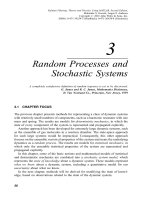
EXAMPLE 3.2: Experiment with Two Dice Consider a toss with two dice in
which one die has come to rest before the other and just enough of its face is visible
to show that it contains either four or ®ve dots. The question is: What is the
probability distribution of the score, given that information?
The probability space for two dice. This example illustrates just how rapidly the
sizes of probability spaces grow with the ``problem size'' (in this case, the number of
dice). For a single die, the sample space has 6 outcomes and the sigma algebra has
64 events. For two dice, the sample space has 36 possible outcomes (6 independent
outcomes for each of two dice) and 2
36
 68, 719, 476, 736 possible events. If each
4
Discovered by the English clergyman and mathematician Thomas Bayes (1702±1761). Conditioning on
impossible events is not de®ned. Note that the conditional probability is based on the assumption that e
c
has occurred. This would seem to imply that e
c
is an event with nonzero probability, which one might
expect from practical applications of Bayes' rule.
64 RANDOM PROCESSES AND STOCHASTIC SYSTEMS
die is fair and their outcomes are independent, then all outcomes with two dice have
probability 
1
6
Â
1
6

1

36
and the probability of any event is the number of outcomes
in the event divided by 36 (the number of outcomes in the sample space). Using the
same notation as the previous (one-die) example, let the outcome from tossing a pair
of dice be represented by an ordered pair (in parentheses) of the outcomes of the ®rst
and second die, respectively. Then the score so
i
; o
j
  do
i
do
j
, where o
i
represents the outcome of the ®rst die and o
j
represents the outcome of the second
die. The corresponding probability distribution function of the score x for two dice is
shown in Figure 3.3a.
The event corresponding to the condition that the ®rst die have either four or ®ve
dots showing contains all outcomes in which o
i
 o
d
or o
e
; which is the set
e
c

fo
d
; o
a
; o
d
; o
b
; o
d
; o
c
; o
d
; o
d
; o
d
; o
e
; o
d
; o
f

o
e
; o
a
; o

e
; o
b
; o
e
; o
c
; o
e
; o
d
; o
e
; o
e
; o
e
; o
f
g;
of 12 outcomes. It has probability pe
c

12
36

1
3
:
Fig. 3.3 Probability distributions of dice scores.

3.2 PROBABILITY AND RANDOM VARIABLES 65
By applying Bayes' rule, the conditional probabilities of all events corresponding
to unique scores can be calculated as shown in Figure 3.4. The corresponding
probability distribution function for two dice with this conditioning is shown in
Figure 3.3b.
3.3 STATISTICAL PROPERTIES OF RANDOM VARIABLES
3.3.1 Expected Values of Random Variables
Expected values. The symbol E is used as an operator on random variables. It is
called the expectancy, expected value,oraverage operator, and the expression
E
x
h f xi is used to denote the expected value of the function f applied to the
ensemble of possible values of the random variable x. The symbol under the E
indicates the random variable (RV) over which the expected value is to be evaluated.
When the RV in question is obvious from context, the symbol underneath the E will
be eliminated. If the argument of the expectancy operator is also obvious from
context, the angular brackets can also be disposed with, using Ex instead of Ehxi, for
example.
Moments. The nth moment of a scalar RV x with probability density p(x)is
de®ned by the formula
Z
n
x
def
E
x
hx
n
i
def


I
I
x
n
px dx: 3:18
Fig. 3.4 Conditional scoring probabilities for two dice.
66 RANDOM PROCESSES AND STOCHASTIC SYSTEMS
The nth central moment of x is de®ned as
m
n
x
def
Ehx À Exi
n
3:19


I
ÀI
x À Ex
n
px dx: 3:20
The ®rst moment of x is called its mean
5
:
Z
1
 Ex 


I
ÀI
xpx dx: 3:21
In general, a function of several arguments such as f (x,y,z) has ®rst moment
Ef x; y; z

I
ÀI

f x; y; zpx; y; z dx dy dz: 3:22
Array Dimensions of Moments. The ®rst moment will be a scalar or a vector,
depending on whether the function f (x, y, z) is scalar or vector valued. Higher order
moments have tensorlike properties, which we can characterize in terms of the
number of subscripts used in de®ning them as data structures. Vectors are singly
subscripted data structures. The higher order moments of vector-valued variates are
successively higher order data structures. That is, the second moments of vector-
valued RVs are matrices (doubly subscripted data structures), and the third-order
moments will be triply subscripted data structures.
These de®nitions of a moment apply to discrete-valued random variables if we
simply substitute summations in place of integrations in the de®nitions.
3.3.2 Functions of Random Variables
A function of RV x is the operation of assigning to each value of x another value, for
example y, according to rule or function. This is represented by
y  f x; 3:23
where x and y are usually called input and output, respectively. The statistical
properties of y in terms of x are, for example,
Ey 

I
ÀI

f xpx dx;
.
.
.
3:24
Ey
n


I
ÀI
f x
n
px dx
when y is scalar. For vector-valued functions y, similar expressions can be shown.
5
We here restrict the order of the moment to the positive integers. The zeroth-order moment would
otherwise always evaluate to 1.
3.3 STATISTICAL PROPERTIES OF RANDOM VARIABLES 67
The probability density of y can be obtained from the density of x. If Equation
3.23 can be solved for x, yielding the unique solution
x  gy: 3:25
Then we have
p
y
y
p
x
gy
@f x

@x



xgy
3:26
where p
y
y and p
x
x are the density functions of y and x, respectively. A function of
two RVs, x, y is the process of assigning to each pair of x, y another value, for
example, z, according to the same rule,
z  f  y; x; 3:27
and similarly functions of n RVs. When x and y in Equation 3.23 are n-dimensional
vectors and if a unique solution for x in terms of y exists,
x  gy; 3:28
Equation 3.26 becomes
p
y
y
p
x
gy
jJj
xgy
; 3:29
where the Jacobian jJjis de®ned as the determinant of the array of partial derivatives
@f
i

=@x
j
:
jJjdet
@f
1
@x
1
@f
1
@x
2
ÁÁÁ
@f
1
@x
n
@f
2
@x
1
@f
2
@x
2
ÁÁÁ
@f
2
@x
n

.
.
.
.
.
.
.
.
.
.
.
.
@f
n
@x
1
@f
n
@x
2
ÁÁÁ
@f
n
@x
n
P
T
T
T
T

T
T
T
T
T
T
T
R
Q
U
U
U
U
U
U
U
U
U
U
U
S
: 3:30
3.4 STATISTICAL PROPERTIES OF RANDOM PROCESSES
3.4.1 Random Processes (RPs)
A RV was de®ned as a function x(s) de®ned for each outcome of an experiment
identi®ed by s. Now if we assign to each outcome s a time function x(t, s), we obtain
68 RANDOM PROCESSES AND STOCHASTIC SYSTEMS
a family of functions called random processes or stochastic processes. A random
process is called discrete if its argument is a discrete variable set as
xk; s; k  1; 2 : 3:31

It is clear that the value of a random process x(t) at any particular time t  t
0
, namely
xt
0
; s, is a random variable [or a random vector if xt
0
; s is vector valued].
3.4.2 Mean, Correlation, and Covariance
Let x(t)beann-vector random process. Its mean
Ext

I
ÀI
xtpxt dxt; 3:32
which can be expressed elementwise as
Ex
i
t

I
ÀI
x
i
tpx
i
t dxt; i  1 n:
For a random sequence, the integral is replaced by a sum.
The correlation of the vector-valued process x(t) is de®ned by
Ehxt

1
x
T
t
2
i 
Ehxt
1
x
1
t
2
i ÁÁÁ Ehx
1
t
1
x
n
t
2
i
.
.
.
.
.
.
.
.
.

Ehx
n
t
1
x
1
t
2
i ÁÁÁ Ehx
n
t
1
x
n
t
2
i
P
T
T
T
R
Q
U
U
U
S
; 3:33
where
Ex

i
t
1
x
j
t
2


I
ÀI

x
i
t
1
x
j
t
2
px
i
t
1
; x
j
t
2
 dx
i

t
1
 dx
j
t
2
: 3:34
The covariance of x(t) is de®ned by
Ehxt
1
ÀExt
1
xt
2
ÀExt
2

T
i
 Ehxt
1
x
T
t
2
i À Ehxt
1
iEhx
T
t

2
i:
3:35
When the process x(t) has zero mean (i.e., Ext0 for all t), its correlation and
covariance are equal.
The correlation matrix of two RPs x(t), an n-vector, and y(t), an m-vector, is given
by an n  m matrix
Ext
1
y
T
t
2
; 3:36
3.4 STATISTICAL PROPERTIES OF RANDOM PROCESSES 69
where
Ex
i
t
1
y
j
t
2


I
ÀI

x

i
t
1
y
j
t
2
px
i
t
1
; y
j
t
2
 dx
i
t
1
 dy
j
t
2
3:37
Similarly, the cross-covariance n  m matrix is
Ehxt
1
ÀExt
1
yt

2
ÀEyt
2

T
i: 3:38
3.4.3 Orthogonal Processes and White Noise
Two RPs x(t) and y(t) are called uncorrelated if their cross-covariance matrix is
identically zero for all t
1
and t
2
:
Ehxt
1
ÀEhxt
1
iyt
2
ÀEhyt
2
i
T
0: 3:39
The processes x(t) and y(t) are called orthogonal if their correlation matrix is
identically zero:
Ehxt
1
y
T

t
2
i  0: 3:40
The random process x(t) is called uncorrelated if
Ehxt
1
ÀEhxt
1
ixt
2
ÀEht
2
i
T
iQt
1
; t
2
dt
1
À t
2
; 3:41
where dt is the Dirac delta ``function''
6
(actually, a generalized function), de®ned
by

b
a

dt dt 
1 if a 0 b;
0 otherwise:
@
3:42
Similarly, a random sequence x
k
is called uncorrelated if
Ehx
k
À Ehx
k
ix
j
À Ehx
j
i
T
iQk; j Dk À j; 3:43
where DÁ is the Kronecker delta function
7
, de®ned by
Dk
1ifk  0
0 otherwise:
@
3:44
A white-noise process or sequence is an example of an uncorrelated process or
sequence.
6

Named for the English physicist Paul Adrien Maurice Dirac (1902±1984).
7
Named for the German mathematician Leopold Kronecker (1823±1891).
70 RANDOM PROCESSES AND STOCHASTIC SYSTEMS
A process x(t) is considered independent if for any choice of distinct times
t
1
; t
2
; t
n
, the random variables xt
1
; xt
2
; ; xt
n
 are independent. That is,
p
xt
1

; ; p
xt
n

s
1
; ; s
n



n
i1
p
xt
i

s
i
: 3:45
Independence (all of the moments) implies no correlation (which restricts attention
to the second moments), but the opposite implication is not true, except in such
special cases as Gaussian processes (see Section 3.2.3). Note that whiteness means
uncorrelated in time rather than independent in time (i.e., including all moments),
although this distinction disappears for the important case of white Gaussian
processes (see Chapter 4).
3.4.4 Strict-Sense and Wide-Sense Stationarity
The random process x(t) (or random sequence x
k
) is called strict-sense stationary if
all its statistics (meaning pxt
1
; xt
2
; ) are invariant with respect to shifts of the
time origin:
px
1
; x

2
; ; x
n
; t
1
; ; t
n

 px
1
; x
2
; ; x
n
; t
1
 e; t
2
 e; ; t
n
 e
3:46
The random process x(t) (or x
k
) is called wide-sense stationary (WSS) (or ``weak-
sense'' stationary) if
Ehxti  c a constant3:47
and
Ehxt
1

x
T
t
2
i  Qt
2
À t
1
Qt; 3:48
where Q is a matrix with each element depending only on the difference t
2
À t
1
 t.
Therefore, when x(t) is stationary in the weak sense, it implies that its ®rst- and
second-order statistics are independent of time origin, while strict stationarity by
de®nition implies that statistics of all orders are independent of the time origin.
3.4.5 Ergodic Random Processes
A process is considered ergodic
8
if all of its statistical parameters, mean, variance,
and so on, can be determined from arbitrarily chosen member functions. A sampled
function x(t) is ergodic if its time-averaged statistics equal the ensemble averages.
8
The term ergodic came originally from the development of statistical mechanics for thermodynamic
systems. It is taken from the Greek words for energy and path. The term was applied by the American
physicist Josiah Willard Gibbs (1839±1903) to the time history (or path) of the state of a thermodynamic
system of constant energy. Gibbs had assumed that a thermodynamic system would eventually take on all
possible states consistent with its energy. It was shown to be impossible from function-theoretic
considerations in the nineteenth century. The so-called ergodic hypothesis of James Clerk Maxwell

(1831±1879) is that the temporal means of a stochastic system are equivalent to the ensemble means. The
concept was given ®rmer mathematical foundations by George David Birkhoff and John von Neumann
around 1930 and by Norbert Wiener in the 1940s.
3.4 STATISTICAL PROPERTIES OF RANDOM PROCESSES 71
3.4.6 Markov Processes and Sequences
An RP x(t) is called a Markov process
9
if its future state distribution, conditioned on
knowledge of its present state, is not improved by knowledge of previous states:
pfxt
i
jxt; t < t
iÀ1
gpfxt
i
jxt
iÀ1
g; 3:49
where the times t
1
< t
2
< t
3
< ÁÁÁ< t
i
:
Similarly, a random sequence (RS) x
k
is called a Markov sequence if

px
i
jx
k
; k i À 1pfx
i
jx
iÀ1
g: 3:50
The solution to a general ®rst-order differential or difference equation with an
independent process (uncorrelated normal RP) as a forcing function is a Markov
process. That is, if x(t) and x
k
are n-vectors satisfying
_
xtFtxtGtwt3:51
or
x
k
 F
kÀ1
x
kÀ1
 G
kÀ1
w
kÀ1
; 3:52
where wt and w
kÀ1

are r-dimensional independent random processes and
sequences, the solutions x(t) and x
k
are then vector Markov processes and sequences,
respectively.
3.4.7 Gaussian Processes
An n-dimensional RP x(t) is called Gaussian (or normal) if its probability density
function is Gaussian, as given by the formulas of Section 3.2.3, with covariance
matrix
P  EhjxtÀEhxtijxtÀEhxti
T
i3:53
for the random variable x.
Gaussian random processes have some useful properties:
1. A Gaussian RP x(t) is WSSÐand stationary in the strict sense.
2. Orthogonal Gaussian RPs are independent.
3. Any linear function of jointly Gaussian RP results in another Gaussian RP.
4. All statistics of a Gaussian RP are completely determined by its ®rst- and
second-order statistics.
9
De®ned by Andrei Andreevich Markov (1856±1922).
72 RANDOM PROCESSES AND STOCHASTIC SYSTEMS
3.4.8 Simulating Multivariate Gaussian Processes
Cholesky decomposition methods are discussed in Chapter 6 and Appendix B.
We show here how these methods can be used to generate uncorrelated pseudo-
random vector sequences with zero mean (or any speci®ed mean) and a speci®ed
covariance P.
There are many programs that will generate pseudorandom sequences of
uncorrelated Gaussian scalars s
i

ji  1; 2; 3; g
È
with zero mean and unit variance:
Ehs
i
iPn0; 1 for all i; 3:54
Ehs
i
s
j
i
0if i T j;
1if i  j
@
3:55
These can be used to generate sequences of Gaussian n-vectors x
k
with mean zero
and covariance I
m
:
u
k
s
nk1
s
nk2
s
nk3
ÁÁÁ s

nk1

T
; 3:56
Ehu
k
i0; 3:57
Ehu
k
u
T
k
iI
n
: 3:58
These vectors, in turn, can be used to generate a sequence of n-vectors w
k
with zero
mean and covariance P. For that purpose, let
CC
T
 P 3:59
be a Cholesky decomposition of P, and let the sequence of n-vectors w
k
be generated
according to the rule
w
k
 Cu
k

: 3:60
Then the sequence of vectors w
0
; w
1
; w
2
; g
È
will have mean
Ehw
k
iCEhu
k
i3:61
 0 3:62
(an n-vector of zeros) and covariance
Ehw
k
w
T
k
iEhCu
k
Cu
k

T
i3:63
 CI

n
C
T
3:64
 P: 3:65
3.4 STATISTICAL PROPERTIES OF RANDOM PROCESSES 73
The same technique can be used to obtain pseudorandom Gaussian vectors with a
given mean v by adding v to each w
k
. These techniques are used in simulation and
Monte Carlo analysis of stochastic systems.
3.4.9 Power Spectral Density
Let x(t) be a zero-mean scalar stationary RP with autocorrelation c
x
t,
Ehxtxt  ti  c
x
t3:66
The power spectral density (PSD) is de®ned as
C
x
o

I
ÀI
c
x
te
Àjot
dt 3:67

and the inverse transform as
c
x
t
1
2p

I
ÀI
C
x
oe
jot
do : 3:68
The following are properties of autocorrelation functions:
1. Autocorrelation functions are symmetrical ( ``even'' functions).
2. An autocorrelation function attains its maximum value at the origin.
3. Its Fourier transform is nonnegative (greater than or equal to zero).
These properties are satis®ed by valid autocorrelation functions.
Setting t  0 in Equation 3.68 gives
E
t
hx
2
ti  c
x
0
1
2p


I
ÀI
C
x
o do: 3:69
Because of property 1 of the autocorrelation function,
C
x
oC
x
Ào; 3:70
that is, the PSD is a symmetric function of frequency.
74 RANDOM PROCESSES AND STOCHASTIC SYSTEMS
EXAMPLE 3.3 If c
x
ts
2
e
Àajtj
, ®nd the associated PSD:
C
x
o

0
ÀI
s
2
e
at

e
Àjot
dt 

I
0
s
2
e
Àat
e
Àjot
dt
 s
2
1
a À jo

1
a  jo


2s
2
a
o
2
 a
2
:

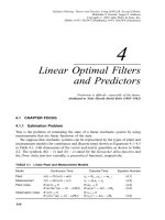
EXAMPLE 3.4 This is an example of a second-order Markov process generated
by passing WSS white noise with zero mean and unit variance through a second-
order ``shaping ®lter'' with the dynamic model of a harmonic resonator. (This is the
same example introduced in Chapter 2 and will be used again in Chapters 4 and 5.)
The transfer function of the dynamic system is
Hs
as  b
s
2
 2zw
n
s  w
2
n
:
De®nitions of z, w
n
, and s are the same as in Example 2.7. The state-space model of
H(s) is given as
_
x
1
t
_
x
2
t
45

01

Àw
2
n
À2zw
n
45
x
1t
x
2
t
45

a
b À 2azw
n
45
wt;
ztx
1
txt:
The general form of the autocorrelation is
c
x
t
s
2
cos y
e
Àzw

n
jtj
cos

1 À z
2
q
w
n
jtjÀy

:
In practice, s
2
, y, z , and w
n
are chosen to ®t empirical data (see Problem 3.13). The
PSD corresponding to the c
x
t will have the form
C
x
w
a
2
w
2
 b
2
w

4
 2w
2
n
2z
2
À 1w
2
 w
4
n
:
(The peak of this PSD will not be at the ``natural'' (undamped) frequency o
n
; but at
the ``resonant'' frequency de®ned in Example 2.6.)
The block diagram corresponding to the state-space model is shown in Figure 3.5.
3.4 STATISTICAL PROPERTIES OF RANDOM PROCESSES 75
The mean power of a scalar random process is given by the equations
E
t
hx
2
ti  lim
T3I

T
ÀT
x
2

t dt 3:71

1
2p

I
ÀI
C
x
o do 3:72
 s
2
: 3:73
The cross power spectral density between an RP x and an RP y is given by the
formula
C
xy
o

I
ÀI
c
xy
te
Àjot
dt 3:74
3.5 LINEAR SYSTEM MODELS OF RANDOM PROCESSES
AND SEQUENCES
Assume that a linear system is given by
yt


I
ÀI
xtht; tdt; 3:75
where x(t) is input and ht; t is the system weighting function (see Figure 3.6). If the
system is time invariant, then Equation 3.75 becomes
yt

I
0
htxt À tdt: 3:76
b
w
∫
∫
Fig. 3.5 Diagram of a second-order Markov process.
Fig. 3.6 Block diagram representation of a linear system.
76 RANDOM PROCESSES AND STOCHASTIC SYSTEMS
This type of integral is called a convolution integral. Manipulation of Equation 3.76
leads to relationships between autocorrelation functions of x(t) and y(t),
c
y
t

I
0
dt
1
ht
1



I
0
dt
2
ht
2
c
x
t  t
1
À t
2
; 3:77
c
xy
t

I
0
ht
1
c
x
t À t
1
dt
1
3:78

and PSD relationships
C
xy
oH joC
x
o; 3:79
C
y
ojH joj
2
C
x
o; 3:80
where H is the system transfer function shown in Figure 3.6, de®ned in Laplace
transform notation as
Hs

I
0
hte
st
dt; 3:81
where s  jo.
3.5.1 Stochastic Differential Equations
for Random Processes
A Note on the Calculus of Stochastic Differential Equations. Differential
equations involving random processes are called stochastic differential equations.
Introducing random processes as inhomogeneous terms in ordinary differential
equations has rami®cations beyond the level of rigor that will be followed here,
but the reader should be aware of them. The problem is that random processes are

not integrable functions in the conventional (Riemann) calculus. The resolution of
this problem requires foundational modi®cations of the calculus to obtain many of
the results presented. The Riemann integral of the ``ordinary'' calculus must be
modi®ed to what is called the Ito
Ã
calculus. The interested reader will ®nd these
issues treated more rigorously in the books by Bucy and Joseph [15] and Ito
Ã
[113].
A linear stochastic differential equation as a model of an RP with initial
conditions has the form
_
xtFtxtGtwtCtut;
ztHtxtvtDtut;
3:82
3.5 LINEAR SYSTEM MODELS OF RANDOM PROCESSES AND SEQUENCES 77
where the variables are de®ned as
xtn Â1 state vector;
zt` Â 1 measurement vector;
utr Â1 deterministic input vector;
Ftn  n time-varying dynamic coefficient matrix;
Ctn Âr time-varying input coupling matrix;
Ht` Ân time-varying measurement sensitivity matrix;
Dt` Âr time-varying output coupling matrix;
Gtn  r time-varying process noise coupling matrix;
wtr  1 zero-mean uncorrelated ``plant noise'' process;
vt` Â 1 zero-mean uncorrelated ``measurement noise'' process
and the expected values as
Ehwti  0;
Ehvti  0;

Ehwt
1
w
T
t
2
i  Qt
1
dt
2
À t
1
;
Ehvt
1
v
T
t
2
i  Rt
1
dt
2
À t
1
:
Ehvt
1
v
T

t
2
i  M t
1
dt
2
À t
1
:
The symbols Q, R, and M represent r Âr, ` Â`, and r  ` matrices, respectively,
and d represents the Dirac delta ``function'' (a measure). The values over time of
the variable x(t) in the differential equation model de®ne vector-valued Markov
processes. This model is a fairly accurate and useful representation for many real-
world processes, including stationary Gaussian and nonstationary Gaussian
processes, depending on the statistical properties of the random variables and the
temporal properties of the deterministic variables. [The function u(t) usually
represents a known control input. For the rest of the discussion in this chapter, we
will assume that ut0.]
EXAMPLE 3.5 Continuing with Example 3.3, let the RP x(t) be a zero-mean
stationary normal RP having autocorrelation
c
x
ts
2
e
Àajtj
: 3:83
The corresponding power spectral density is
C
x

o
2s
2
a
o
2
 a
2
: 3:84
78 RANDOM PROCESSES AND STOCHASTIC SYSTEMS
This type of RP can be modeled as the output of a linear system with input w(t), a
zero-mean white Gaussian noise with PSD equal to unity. Using Equation 3.80, one
can derive the transfer function Hjo for the following model:
wt
ÀÀÀÀÀÀÀÀÀÀÀ3
Hjo
xt
ÀÀÀÀÀÀÀÀÀÀÀ3
HjoHÀjo

2a
p
s
a  jo
Á

2a
p
s
a À jo

:
C
w
o1
c
w
tdt
C
x
o
c
x
t
Take the stable portion of this system transfer function as
Hs

2a
p
s
s  a
; 3:85
which can be represented as
xs
ws


2a
p
s
s  a

; 3:86
By taking the inverse Laplace transform of both sides of this last equation, one can
obtain the following sequence of equations:
_
xtaxt

2a
p
swt;
_
xtÀaxt

2a
p
swt;
ztxt;
with s
2
x
0s
2
. The parameter 1=a is called the correlation time of the process.
The block diagram representation of the process in Example 3.5 is shown in Table
3.1. This is called a shaping ®lter. Some other examples of differential equation
models are also given in Table 3.1.
3.5.2 Discrete Model of a Random Sequence
A vector discrete-time recursive equation for modeling a random sequence (RS) with
initial conditions can be given in the form
x
k

 F
kÀ1
x
kÀ1
 G
kÀ1
w
kÀ1
 G
kÀ1
u
kÀ1
;
z
k
 H
k
x
k
 v
k
 D
k
u
k
: 3:87
3.5 LINEAR SYSTEM MODELS OF RANDOM PROCESSES AND SEQUENCES 79
TABLE 3.1 System Models of Random Processes
Random Process Autocorrelation
Function and

Power Spectral
Density
Shaping
Filter
Diagram
State-Space
Formulation
White noise c
x
ts
2
d
2
t None Always treated as
c
x
os
2
measurement noise
Random walk c
x
tundefined
_
x  w t
c
x
oGs
2
=o
2

s
2
x
00
Random constant c
x
ts
2
None
_
x  0
c
x
o2ps
2
do s
2
x
0s
2
Sinusoid c
x
ts
2
coso
0
t
_
x 
01

Ào
2
0
0
!
x
C
x
ops
2
do Ào
0

ps
2
do o
0

P0
s
2
0
00
!
Exponentially correlated c
x
ts
2
e
Àajtj

C
x
o
2s
a
a
o
2
 a
2
_x Àax s

2a
p
w t
s
2
x
0s
2
1
a
 correlation time
80 RANDOM PROCESSES AND STOCHASTIC SYSTEMS