Tài liệu Ten Principles of Economics - Part 40 docx

CHAPTER 18 THE MARKETS FOR THE FACTORS OF PRODUCTION 403
WHAT CAUSES THE LABOR DEMAND CURVE TO SHIFT?
We now understand the labor demand curve: It is nothing more than a reflection
of the value of marginal product of labor. With this insight in mind, let’s consider
a few of the things that might cause the labor demand curve to shift.
The Output Price The value of the marginal product is marginal product
times the price of the firm’s output. Thus, when the output price changes, the
value of the marginal product changes, and the labor demand curve shifts. An in-
crease in the price of apples, for instance, raises the value of the marginal product
of each worker that picks apples and, therefore, increases labor demand from the
firms that supply apples. Conversely, a decrease in the price of apples reduces the
value of the marginal product and decreases labor demand.
Technological Change Between 1968 and 1998, the amount of output
a typical U.S. worker produced in an hour rose by 57 percent. Why? The most
In Chapter 14 we saw how
a competitive, profit-maximizing
firm decides how much of its
output to sell: It chooses the
quantity of output at which the
price of the good equals the
marginal cost of production. We
have just seen how such a firm
decides how much labor to
hire: It chooses the quantity of
labor at which the wage equals
the value of the marginal prod-
uct. Because the production
function links the quantity of inputs to the quantity of output,
you should not be surprised to learn that the firm’s decision
about input demand is closely linked to its decision about
output supply. In fact, these two decisions are two sides of

the same coin.
To see this relationship more fully, let’s consider how
the marginal product of labor (MPL) and marginal cost (MC)
are related. Suppose an additional worker costs $500 and
has a marginal product of 50 bushels of apples. In this
case, producing 50 more bushels costs $500; the marginal
cost of a bushel is $500/50, or $10. More generally, if W
is the wage, and an extra unit of labor produces MPL units
of output, then the marginal cost of a unit of output is
MC ϭ W/MPL.
This analysis shows that diminishing marginal product
is closely related to increasing marginal cost. When our ap-
ple orchard grows crowded with workers, each additional
worker adds less to the production of apples (MPL falls).
Similarly, when the apple firm is producing a large quantity
of apples, the orchard is already crowded with workers, so it
is more costly to produce an additional bushel of apples
(MC rises).
Now consider our criterion for profit maximization. We
determined earlier that a profit-maximizing firm chooses the
quantity of labor so that the value of the marginal product
(P ϫ MPL) equals the wage (W). We can write this mathe-
matically as
P ϫ MPL ϭ W.
If we divide both sides of this equation by MPL, we obtain
P ϭ W/MPL.
We just noted that W/MPL equals marginal cost MC. There-
fore, we can substitute to obtain
P ϭ MC.
This equation states that the price of the firm’s output is

equal to the marginal cost of producing a unit of output.
Thus, when a competitive firm hires labor up to the point at
which the value of the marginal product equals the wage, it
also produces up to the point at which the price equals mar-
ginal cost. Our analysis of labor demand in this chapter is
just another way of looking at the production decision we
first saw in Chapter 14.
FYI
Input Demand
and Output
Supply: Two
Sides of the
Same Coin
404 PART SIX THE ECONOMICS OF LABOR MARKETS
important reason is technological progress: Scientists and engineers are constantly
figuring out new and better ways of doing things. This has profound implications
for the labor market. Technological advance raises the marginal product of labor,
which in turn increases the demand for labor. Such technological advance explains
persistently rising employment in face of rising wages: Even though wages (ad-
justed for inflation) increased by 62 percent over these three decades, firms
nonetheless increased by 72 percent the number of workers they employed.
The Supply of Other Factors The quantity available of one factor of
production can affect the marginal product of other factors. A fall in the supply of
ladders, for instance, will reduce the marginal product of apple pickers and thus
the demand for apple pickers. We consider this linkage among the factors of pro-
duction more fully later in the chapter.
QUICK QUIZ: Define marginal product of labor and value of the marginal
product of labor. ◆ Describe how a competitive, profit-maximizing firm
decides how many workers to hire.
THE SUPPLY OF LABOR

Having analyzed labor demand in detail, let’s turn to the other side of the market
and consider labor supply. A formal model of labor supply is included in Chapter
21, where we develop the theory of household decisionmaking. Here we discuss
briefly and informally the decisions that lie behind the labor supply curve.
THE TRADEOFF BETWEEN WORK AND LEISURE
One of the Ten Principles of Economics in Chapter 1 is that people face tradeoffs.
Probably no tradeoff is more obvious or more important in a person’s life than the
tradeoff between work and leisure. The more hours you spend working, the fewer
hours you have to watch TV, have dinner with friends, or pursue your favorite
hobby. The tradeoff between labor and leisure lies behind the labor supply curve.
Another one of the Ten Principles of Economics is that the cost of something is
what you give up to get it. What do you give up to get an hour of leisure? You give
up an hour of work, which in turn means an hour of wages. Thus, if your wage is
$15 per hour, the opportunity cost of an hour of leisure is $15. And when you get a
raise to $20 per hour, the opportunity cost of enjoying leisure goes up.
The labor supply curve reflects how workers’ decisions about the labor–leisure
tradeoff respond to a change in that opportunity cost. An upward-sloping labor
supply curve means that an increase in the wage induces workers to increase the
quantity of labor they supply. Because time is limited, more hours of work means
that workers are enjoying less leisure. That is, workers respond to the increase in
the opportunity cost of leisure by taking less of it.
It is worth noting that the labor supply curve need not be upward sloping.
Imagine you got that raise from $15 to $20 per hour. The opportunity cost of
CHAPTER 18 THE MARKETS FOR THE FACTORS OF PRODUCTION 405
leisure is now greater, but you are also richer than you were before. You might
decide that with your extra wealth you can now afford to enjoy more leisure;
in this case, your labor supply curve would slope backwards. In Chapter 21, we
discuss this possibility in terms of conflicting effects on your labor-supply deci-
sion (called income and substitution effects). For now, we ignore the possibility of
backward-sloping labor supply and assume that the labor supply curve is upward

sloping.
WHAT CAUSES THE LABOR SUPPLY CURVE TO SHIFT?
The labor supply curve shifts whenever people change the amount they want to
work at a given wage. Let’s now consider some of the events that might cause such
a shift.
Changes in Tastes In 1950, 34 percent of women were employed at paid
jobs or looking for work. In 1998, the number had risen to 60 percent. There are, of
course, many explanations for this development, but one of them is changing
tastes, or attitudes toward work. A generation or two ago, it was the norm for
women to stay at home while raising children. Today, family sizes are smaller, and
more mothers choose to work. The result is an increase in the supply of labor.
Changes in Alternative Opportunities The supply of labor in any
one labor market depends on the opportunities available in other labor markets. If
the wage earned by pear pickers suddenly rises, some apple pickers may choose to
switch occupations. The supply of labor in the market for apple pickers falls.
Immigration Movements of workers from region to region, or country to
country, is an obvious and often important source of shifts in labor supply. When
immigrants come to the United States, for instance, the supply of labor in the
United States increases and the supply of labor in the immigrants’ home countries
contracts. In fact, much of the policy debate about immigration centers on its effect
on labor supply and, thereby, equilibrium in the labor market.
QUICK QUIZ: Who has a greater opportunity cost of enjoying leisure—a
janitor or a brain surgeon? Explain. Can this help explain why doctors work
such long hours?
EQUILIBRIUM IN THE LABOR MARKET
So far we have established two facts about how wages are determined in compet-
itive labor markets:
◆ The wage adjusts to balance the supply and demand for labor.
◆ The wage equals the value of the marginal product of labor.
406 PART SIX THE ECONOMICS OF LABOR MARKETS

At first, it might seem surprising that the wage can do both these things at once. In
fact, there is no real puzzle here, but understanding why there is no puzzle is an
important step to understanding wage determination.
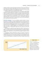
Figure 18-4 shows the labor market in equilibrium. The wage and the quantity
of labor have adjusted to balance supply and demand. When the market is in this
equilibrium, each firm has bought as much labor as it finds profitable at the equi-
librium wage. That is, each firm has followed the rule for profit maximization: It
has hired workers until the value of the marginal product equals the wage. Hence,
the wage must equal the value of marginal product of labor once it has brought
supply and demand into equilibrium.
This brings us to an important lesson: Any event that changes the supply or de-
mand for labor must change the equilibrium wage and the value of the marginal product by
the same amount, because these must always be equal. To see how this works, let’s con-
sider some events that shift these curves.
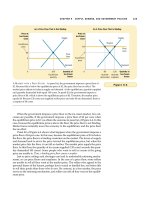
SHIFTS IN LABOR SUPPLY
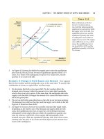
Suppose that immigration increases the number of workers willing to pick apples.
As Figure 18-5 shows, the supply of labor shifts to the right from S
1
to S
2
. At the
initial wage W
1
, the quantity of labor supplied now exceeds the quantity de-
manded. This surplus of labor puts downward pressure on the wage of apple pick-
ers, and the fall in the wage from W
1
to W
2
in turn makes it profitable for firms to

hire more workers. As the number of workers employed in each apple orchard
rises, the marginal product of a worker falls, and so does the value of the marginal
product. In the new equilibrium, both the wage and the value of the marginal
product of labor are lower than they were before the influx of new workers.
Wage
(price of
labor)
Equilibrium
wage,
W
0
Quantity of
Labor
Equilibrium
employment,
L
Supply
Demand
Figure 18-4
EQUILIBRIUM IN A LABOR
MARKET. Like all prices, the
price of labor (the wage) depends
on supply and demand. Because
the demand curve reflects the
value of the marginal product of
labor, in equilibrium workers
receive the value of their
marginal contribution to the
production of goods and services.
CHAPTER 18 THE MARKETS FOR THE FACTORS OF PRODUCTION 407

An episode from Israel illustrates how a shift in labor supply can alter the
equilibrium in a labor market. During most of the 1980s, many thousands of Pale-
stinians regularly commuted from their homes in the Israeli-occupied West Bank
and Gaza Strip to jobs in Israel, primarily in the construction and agriculture
industries. In 1988, however, political unrest in these occupied areas induced the
Israeli government to take steps that, as a by-product, reduced this supply of
workers. Curfews were imposed, work permits were checked more thoroughly,
and a ban on overnight stays of Palestinians in Israel was enforced more rigor-
ously. The economic impact of these steps was exactly as theory predicts: The
number of Palestinians with jobs in Israel fell by half, while those who continued
to work in Israel enjoyed wage increases of about 50 percent. With a reduced num-
ber of Palestinian workers in Israel, the value of the marginal product of the re-
maining workers was much higher.
SHIFTS IN LABOR DEMAND
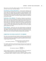
Now suppose that an increase in the popularity of apples causes their price to rise.
This price increase does not change the marginal product of labor for any given
number of workers, but it does raise the value of the marginal product. With a
higher price of apples, hiring more apple pickers is now profitable. As Figure 18-6
shows, when the demand for labor shifts to the right from D
1
to D
2
, the equilib-
rium wage rises from W
1
to W
2
, and equilibrium employment rises from L
1
to L

2
.
Once again, the wage and the value of the marginal product of labor move
together.
This analysis shows that prosperity for firms in an industry is often linked
to prosperity for workers in that industry. When the price of apples rises, apple
Wage
(price of
labor)
W
2
W
1
0
Quantity of
Labor
L
2
L
1
Supply,
S
1
Demand
2. . . . reduces
the wage . . .
3. . . . and raises employment.
1. An increase in
labor supply . . .
S

2
Figure 18-5
ASHIFT IN LABOR SUPPLY.
When labor supply increases
from S
1
to S
2
, perhaps because of
an immigration of new workers,
the equilibrium wage falls from
W
1
to W
2
. At this lower wage,
firms hire more labor, so
employment rises from L
1
to L
2
.
The change in the wage reflects a
change in the value of the
marginal product of labor: With
more workers, the added output
from an extra worker is smaller.
408 PART SIX THE ECONOMICS OF LABOR MARKETS
CASE STUDY PRODUCTIVITY AND WAGES
One of the Ten Principles of Economics in Chapter 1 is that our standard of living

depends on our ability to produce goods and services. We can now see how this
principle works in the market for labor. In particular, our analysis of labor de-
mand shows that wages equal productivity as measured by the value of the
marginal product of labor. Put simply, highly productive workers are highly
paid, and less productive workers are less highly paid.
This lesson is key to understanding why workers today are better off than
workers in previous generations. Table 18-2 presents some data on growth in
productivity and growth in wages (adjusted for inflation). From 1959 to 1997,
productivity as measured by output per hour of work grew about 1.8 percent
per year; at this rate, productivity doubles about every 40 years. Over this pe-
riod, wages grew at a similar rate of 1.7 percent per year.
producers make greater profit, and apple pickers earn higher wages. When the
price of apples falls, apple producers earn smaller profit, and apple pickers earn
lower wages. This lesson is well known to workers in industries with highly
volatile prices. Workers in oil fields, for instance, know from experience that their
earnings are closely linked to the world price of crude oil.
From these examples, you should now have a good understanding of how
wages are set in competitive labor markets. Labor supply and labor demand to-
gether determine the equilibrium wage, and shifts in the supply or demand curve
for labor cause the equilibrium wage to change. At the same time, profit maxi-
mization by the firms that demand labor ensures that the equilibrium wage always
equals the value of the marginal product of labor.
Wage
(price of
labor)
W
1
W
2
0

Quantity of
Labor
L
1
L
2
Supply
Demand,
D
1
2. . . . increases
the wage . . .
3. . . . and increases employment.
1. An increase in
labor demand . . .
D
2
Figure 18-6
ASHIFT IN LABOR DEMAND.
When labor demand increases
from D
1
to D
2
, perhaps because of
an increase in the price of the
firms’ output, the equilibrium
wage rises from W
1
to W

2
, and
employment rises from L
1
to L
2
.
Again, the change in the wage
reflects a change in the value of
the marginal product of labor:
With a higher output price, the
added output from an extra
worker is more valuable.
CHAPTER 18 THE MARKETS FOR THE FACTORS OF PRODUCTION 409
Table 18-2 also shows that, beginning around 1973, growth in productivity
slowed from 2.9 to 1.1 percent per year. This 1.8 percentage-point slowdown in
productivity coincided with a slowdown in wage growth of 1.9 percentage
points. Because of this productivity slowdown, workers in the 1980s and 1990s
did not experience the same rapid growth in living standards that their parents
enjoyed. A slowdown of 1.8 percentage points might not seem large, but accu-
mulated over many years, even a small change in a growth rate is significant. If
productivity and wages had grown at the same rate since 1973 as they did pre-
viously, workers’ earnings would now be about 50 percent higher than they are.
The link between productivity and wages also sheds light on international
experience. Table 18-3 presents some data on productivity growth and wage
growth for a representative group of countries, ranked in order of their produc-
tivity growth. Although these international data are far from precise, a close link
between the two variables is apparent. In South Korea, Hong Kong, and Singa-
pore, productivity has grown rapidly, and so have wages. In Mexico, Argentina,
and Iran, productivity has fallen, and so have wages. The United States falls

about in the middle of the distribution: By international standards, U.S. pro-
ductivity growth and wage growth have been neither exceptionally bad nor ex-
ceptionally good.
What causes productivity and wages to vary so much over time and across
countries? A complete answer to this question requires an analysis of long-run
economic growth, a topic beyond the scope of this chapter. We can, however,
briefly note three key determinants of productivity:
◆ Physical capital: When workers work with a larger quantity of equipment
and structures, they produce more.
◆ Human capital: When workers are more educated, they produce more.
◆ Technological knowledge: When workers have access to more sophisticated
technologies, they produce more.
Physical capital, human capital, and technological knowledge are the ulti-
mate sources of most of the differences in productivity, wages, and standards of
living.
Table 18-2
PRODUCTIVITY AND WAGE
GROWTH IN THE UNITED STATES
GROWTH RATE GROWTH RATE
TIME PERIOD OF PRODUCTIVITY OF REAL WAGES
1959–1997 1.8 1.7
1959–1973 2.9 2.9
1973–1997 1.1 1.0
S
OURCE: Economic Report of the President 1999, table B-49, p. 384. Growth in productivity is measured here
as the annualized rate of change in output per hour in the nonfarm business sector. Growth in real
wages is measured as the annualized change in compensation per hour in the nonfarm business sector
divided by the implicit price deflator for that sector. These productivity data measure average
productivity—the quantity of output divided by the quantity of labor—rather than marginal
productivity, but average and marginal productivity are thought to move closely together.

410 PART SIX THE ECONOMICS OF LABOR MARKETS
QUICK QUIZ: How does an immigration of workers affect labor supply,
labor demand, the marginal product of labor, and the equilibrium wage?
THE OTHER FACTORS OF PRODUCTION:
LAND AND CAPITAL
We have seen how firms decide how much labor to hire and how these decisions
determine workers’ wages. At the same time that firms are hiring workers, they
are also deciding about other inputs to production. For example, our apple-
producing firm might have to choose the size of its apple orchard and the number
of ladders to make available to its apple pickers. We can think of the firm’s factors
of production as falling into three categories: labor, land, and capital.
The meaning of the terms labor and land is clear, but the definition of capital is
somewhat tricky. Economists use the term capital to refer to the stock of equip-
ment and structures used for production. That is, the economy’s capital represents
the accumulation of goods produced in the past that are being used in the present
to produce new goods and services. For our apple firm, the capital stock includes
the ladders used to climb the trees, the trucks used to transport the apples, the
buildings used to store the apples, and even the trees themselves.
EQUILIBRIUM IN THE MARKETS FOR LAND AND CAPITAL
What determines how much the owners of land and capital earn for their con-
tribution to the production process? Before answering this question, we need to
Table 18-3
PRODUCTIVITY AND WAGE
GROWTH AROUND THE WORLD
GROWTH RATE GROWTH RAT E
COUNTRY OF PRODUCTIVITY OF REAL WAGES
South Korea 8.5 7.9
Hong Kong 5.5 4.9
Singapore 5.3 5.0
Indonesia 4.0 4.4

Japan 3.6 2.0
India 3.1 3.4
United Kingdom 2.4 2.4
United States 1.7 0.5
Brazil 0.4 Ϫ2.4
Mexico Ϫ0.2 Ϫ3.0
Argentina Ϫ0.9 Ϫ1.3
Iran Ϫ1.4 Ϫ7.9
SOURCE: World Development Report 1994, table 1, pp. 162–163, and table 7, pp. 174–175. Growth in
productivity is measured here as the annualized rate of change in gross national product per person
from 1980 to 1992. Growth in wages is measured as the annualized change in earnings per employee in
manufacturing from 1980 to 1991.
capital
the equipment and structures used to
produce goods and services
CHAPTER 18 THE MARKETS FOR THE FACTORS OF PRODUCTION 411
distinguish between two prices: the purchase price and the rental price. The pur-
chase price of land or capital is the price a person pays to own that factor of pro-
duction indefinitely. The rental price is the price a person pays to use that factor for
a limited period of time. It is important to keep this distinction in mind because, as
we will see, these prices are determined by somewhat different economic forces.
Having defined these terms, we can now apply the theory of factor demand
we developed for the labor market to the markets for land and capital. The wage
is, after all, simply the rental price of labor. Therefore, much of what we have
learned about wage determination applies also to the rental prices of land and cap-
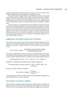
ital. As Figure 18-7 illustrates, the rental price of land, shown in panel (a), and the
rental price of capital, shown in panel (b), are determined by supply and demand.
Moreover, the demand for land and capital is determined just like the demand for
labor. That is, when our apple-producing firm is deciding how much land and
how many ladders to rent, it follows the same logic as when deciding how many

workers to hire. For both land and capital, the firm increases the quantity hired un-
til the value of the factor’s marginal product equals the factor’s price. Thus, the de-
mand curve for each factor reflects the marginal productivity of that factor.
We can now explain how much income goes to labor, how much goes to
landowners, and how much goes to the owners of capital. As long as the firms
using the factors of production are competitive and profit-maximizing, each fac-
tor’s rental price must equal the value of the marginal product for that factor.
Labor, land, and capital each earn the value of their marginal contribution to the produc-
tion process.
Now consider the purchase price of land and capital. The rental price and the
purchase price are obviously related: Buyers are willing to pay more to buy a piece
of land or capital if it produces a valuable stream of rental income. And, as we
Quantity of
Land
0
Rental
Price of
Land
P
Q
Demand
Supply
Demand
Supply
Quantity of
Capital
0
Rental
Price of
Capital

Q
P
(a) The Market for Land (b) The Market for Capital
Figure 18-7
THE MARKETS FOR LAND AND CAPITAL. Supply and demand determine the
compensation paid to the owners of land, as shown in panel (a), and the compensation
paid to the owners of capital, as shown in panel (b). The demand for each factor, in turn,
depends on the value of the marginal product of that factor.
412 PART SIX THE ECONOMICS OF LABOR MARKETS
have just seen, the equilibrium rental income at any point in time equals the value
of that factor’s marginal product. Therefore, the equilibrium purchase price of a
piece of land or capital depends on both the current value of the marginal product
and the value of the marginal product expected to prevail in the future.
LINKAGES AMONG THE FACTORS OF PRODUCTION
We have seen that the price paid to any factor of production—labor, land, or capi-
tal—equals the value of the marginal product of that factor. The marginal product
of any factor, in turn, depends on the quantity of that factor that is available. Be-
cause of diminishing returns, a factor in abundant supply has a low marginal
product and thus a low price, and a factor in scarce supply has a high marginal
product and a high price. As a result, when the supply of a factor falls, its equilib-
rium factor price rises.
When the supply of any factor changes, however, the effects are not limited to
the market for that factor. In most situations, factors of production are used to-
gether in a way that makes the productivity of each factor dependent on the quan-
tities of the other factors available to be used in the production process. As a result,
a change in the supply of any one factor alters the earnings of all the factors.
For example, suppose that a hurricane destroys many of the ladders that
workers use to pick apples from the orchards. What happens to the earnings of the
various factors of production? Most obviously, the supply of ladders falls and,
Labor income is an easy con-

cept to understand: It is the
paycheck that workers get from
their employers. The income
earned by capital, however, is
less obvious.
In our analysis, we have
been implicitly assuming that
households own the economy’s
stock of capital—ladders, drill
presses, warehouses, etc.—
and rent it to the firms that use
it. Capital income, in this case,
is the rent that households receive for the use of their capi-
tal. This assumption simplified our analysis of how capital
owners are compensated, but it is not entirely realistic. In
fact, firms usually own the capital they use and, therefore,
they receive the earnings from this capital.
These earnings from capital, however, eventually get
paid to households. Some of the earnings are paid in the
form of interest to those households who have lent money
to firms. Bondholders and bank depositors are two exam-
ples of recipients of interest. Thus, when you receive inter-
est on your bank account, that income is part of the econ-
omy’s capital income.
In addition, some of the earnings from capital are paid
to households in the form of dividends. Dividends are pay-
ments by a firm to the firm’s stockholders. A stockholder is
a person who has bought a share in the ownership of the
firm and, therefore, is entitled to share in the firm’s profits.
A firm does not have to pay out all of its earnings to

households in the form of interest and dividends. Instead, it
can retain some earnings within the firm and use these
earnings to buy additional capital. Although these retained
earnings do not get paid to the firm’s stockholders, the
stockholders benefit from them nonetheless. Because re-
tained earnings increase the amount of capital the firm
owns, they tend to increase future earnings and, thereby,
the value of the firm’s stock.
These institutional details are interesting and impor-
tant, but they do not alter our conclusion about the income
earned by the owners of capital. Capital is paid according to
the value of its marginal product, regardless of whether this
income gets transmitted to households in the form of inter-
est or dividends or whether it is kept within firms as re-
tained earnings.
FYI
What Is
Capital Income?