Tài liệu Ten Principles of Economics - Part 5 ppt

CHAPTER 2 THINKING LIKE AN ECONOMIST 43
variables constant, we know that changes in the price of novels cause changes in
the quantity Emma demands. Remember, however, that our demand curve came
from a hypothetical example. When graphing data from the real world, it is often
more difficult to establish how one variable affects another.
The first problem is that it is difficult to hold everything else constant when
measuring how one variable affects another. If we are not able to hold variables
constant, we might decide that one variable on our graph is causing changes in the
other variable when actually those changes are caused by a third omitted variable
not pictured on the graph. Even if we have identified the correct two variables to
look at, we might run into a second problem—reverse causality. In other words, we
might decide that A causes B when in fact B causes A. The omitted-variable and
reverse-causality traps require us to proceed with caution when using graphs to
draw conclusions about causes and effects.
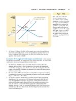
Omitted Variables
To see how omitting a variable can lead to a decep-
tive graph, let’s consider an example. Imagine that the government, spurred by
public concern about the large number of deaths from cancer, commissions an ex-
haustive study from Big Brother Statistical Services, Inc. Big Brother examines
many of the items found in people’s homes to see which of them are associated
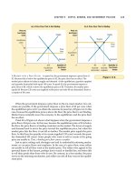
with the risk of cancer. Big Brother reports a strong relationship between two vari-
ables: the number of cigarette lighters that a household owns and the prob-
ability that someone in the household will develop cancer. Figure 2A-6 shows this
relationship.
What should we make of this result? Big Brother advises a quick policy re-
sponse. It recommends that the government discourage the ownership of cigarette
lighters by taxing their sale. It also recommends that the government require
warning labels: “Big Brother has determined that this lighter is dangerous to your
health.”
In judging the validity of Big Brother’s analysis, one question is paramount:
Has Big Brother held constant every relevant variable except the one under con-

sideration? If the answer is no, the results are suspect. An easy explanation for Fig-
ure 2A-6 is that people who own more cigarette lighters are more likely to smoke
cigarettes and that cigarettes, not lighters, cause cancer. If Figure 2A-6 does not
Risk of
Cancer
Number of Lighters in House
0
Figure 2A-6
G
RAPH WITH AN
O
MITTED
V
ARIABLE
. The upward-sloping
curve shows that members of
households with more cigarette
lighters are more likely to
develop cancer. Yet we should
not conclude that ownership of
lighters causes cancer because the
graph does not take into account
the number of cigarettes smoked.
44 PART ONE INTRODUCTION
hold constant the amount of smoking, it does not tell us the true effect of owning
a cigarette lighter.
This story illustrates an important principle: When you see a graph being used
to support an argument about cause and effect, it is important to ask whether the
movements of an omitted variable could explain the results you see.
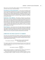
Reverse Causality

Economists can also make mistakes about causality
by misreading its direction. To see how this is possible, suppose the Association
of American Anarchists commissions a study of crime in America and arrives
at Figure 2A-7, which plots the number of violent crimes per thousand people
in major cities against the number of police officers per thousand people. The an-
archists note the curve’s upward slope and argue that because police increase
rather than decrease the amount of urban violence, law enforcement should be
abolished.
If we could run a controlled experiment, we would avoid the danger of re-
verse causality. To run an experiment, we would set the number of police officers
in different cities randomly and then examine the correlation between police and
crime. Figure 2A-7, however, is not based on such an experiment. We simply ob-
serve that more dangerous cities have more police officers. The explanation for this
may be that more dangerous cities hire more police. In other words, rather than
police causing crime, crime may cause police. Nothing in the graph itself allows us
to establish the direction of causality.
It might seem that an easy way to determine the direction of causality is to
examine which variable moves first. If we see crime increase and then the police
force expand, we reach one conclusion. If we see the police force expand and then
crime increase, we reach the other. Yet there is also a flaw with this approach:
Often people change their behavior not in response to a change in their present
conditions but in response to a change in their expectations of future conditions.
A city that expects a major crime wave in the future, for instance, might well hire
more police now. This problem is even easier to see in the case of babies and mini-
vans. Couples often buy a minivan in anticipation of the birth of a child. The
Violent
Crimes
(per 1,000
people)
Police Officers

(per 1,000 people)
0
Figure 2A-7
G
RAPH
S
UGGESTING
R
EVERSE
C
AUSALITY
. The upward-
sloping curve shows that cities
with a higher concentration of
police are more dangerous.
Yet the graph does not tell us
whether police cause crime or
crime-plagued cities hire more
police.
CHAPTER 2 THINKING LIKE AN ECONOMIST 45
minivan comes before the baby, but we wouldn’t want to conclude that the sale
of minivans causes the population to grow!
There is no complete set of rules that says when it is appropriate to draw
causal conclusions from graphs. Yet just keeping in mind that cigarette lighters
don’t cause cancer (omitted variable) and minivans don’t cause larger fam-
ilies (reverse causality) will keep you from falling for many faulty economic
arguments.

IN THIS CHAPTER
YOU WILL . . .

See how comparative
advantage explains
the gains from trade
Consider how
everyone can benefit
when people trade
with one another
Learn the meaning of
absolute advantage
and comparative
advantage
Apply the theory of
comparative
advantage to
everyday life and
national policy
Consider your typical day. You wake up in the morning, and you pour yourself
juice from oranges grown in Florida and coffee from beans grown in Brazil. Over
breakfast, you watch a news program broadcast from New York on your television
made in Japan. You get dressed in clothes made of cotton grown in Georgia and
sewn in factories in Thailand. You drive to class in a car made of parts manufac-
tured in more than a dozen countries around the world. Then you open up your
economics textbook written by an author living in Massachusetts, published by a
company located in Texas, and printed on paper made from trees grown in Oregon.
Every day you rely on many people from around the world, most of whom you
do not know, to provide you with the goods and services that you enjoy. Such inter-
dependence is possible because people trade with one another. Those people who
provide you with goods and services are not acting out of generosity or concern for
your welfare. Nor is some government agency directing them to make what you
INTERDEPENDENCE AND THE

GAINS FROM TRADE
47