Tài liệu Kinh tế ứng dụng_ Lecture 2: Simple Regression Model ppt

Applied Econometrics Simple Linear Regression Model
1
Applied Econometrics
Lecture 2: Simple Regression Model

‘It does require maturity to realize that models are to be used but not to be believed’
HENRI THEIL, Principles of Econometrics


1) Assumptions of the two-variable linear regression model

The estimation process begins by assuming or hypothesizing that the least squares linear regression
model (drawn from a sample) is valid. The formal two-variable linear regression model is based on
the following assumptions:

(1) The population regression is adequately represented by a straight line: E(Y
i
) = μ(X
i
) = β
0
+ β
1
X
i

(2) The error terms have zero mean: E(∈
i
) = 0
(3) A constant variance (homoscedasticity): V(∈
i

) = σ
2

(4) Zero covariance (no correlation): E(∈
i
, ∈
j
) = 0 for all i ≠ j
(5) X is non-stochastic, implying that E(X
i
, ∈
i
) = 0

2) Least squares estimation
The sample regression model can be written as follows:
Y
i
= b
0
+ b
1
X
i
+ e
i

Its least squared estimators b
0
and b

1
are obtained by minimizing the sum of squared residual with
respect to b
0
and b
1

∑e
i
2
= ∑(Y
i
– b
0
– b
1
X
i
)
2
→ min
The resulting estimators of b
0
and b
1
are then given by:
()
(
)
∑⎟

⎠
⎞
⎜
⎝
⎛
−
∑
−−
=
=
=
n
1i
2
n
1i
ii
1
X
X
i
Y
Y
X
X
b


X
b

Y
b
10
−=

3) Analysis of Variances
The least squared regression splits the variation in the Y variable into two components: the explained
variation due to the variation in X
i
and the residual variation
TSS = RSS + ESS
Written by Nguyen Hoang Bao May 20, 2004
Applied Econometrics Simple Linear Regression Model
2

(
∑
−
=
n
i
i
YY
1
2
)
(
)
∑
−

=
n
i
i
Y
Y
1
2
ˆ
(
)
∑
−
=
n
i
i
i
Y
Y
1
2
ˆ
= +
where
TSS is the total sum of squares, which is observed in the dependent variable Y
RSS is the residual sum of squares
ESS is the explanatory sum of squares, which is the variation of the predicted values (b
0
+ b

1
X)

The coefficient of determination, which measures the goodness of fit of the estimated sample
regression:
R
2
= ESS/TSS
0 ≤ R
2
≤ +1

Because the explained variation cannot exceed the total variation, the maximum value of R
2
is one;
that is, 100 percent of the variation is explained or accounted for. Conversely, its minimum value is
zero, which implies that none of the variation in the dependent variable is explained by the
independent variable. There may also be spurious correlation, especially using time-series data.

The correlation coefficient (r) can be calculated as follows:
()
() ()
()()
∑∑
−−
∑
−−
==
==
=

⎟
⎟
⎠
⎞
⎜
⎜
⎝
⎛
⎟
⎟
⎠
⎞
⎜
⎜
⎝
⎛
n
1i
n
1i
22
n
1i
Y
Y
i
n
1
X
X

i
n
1
Y
Y
i
X
X
i
n
1
YVARXVAR
Y)X,COV
r

-1 ≤ r ≤ +1

Note that values close to ±1 indicate very strong relationships, those close to zero indicate very weak
relationships. Now that we have r, how do we know if it is significant different from zero? We must
first convert our t into a value of calculated-t using the following formulae:

The hypothesized value of r is given by: H
0
: r = 0

r1
2n
rt
2
calculated

−
−
=

If t
calculated
> t
critical value
(0.05; n-2): We reject the hypothesis
If t
calculated
≤ t
critical value
(0.05; n-2): We maintain the hypothesis
High correlation do not provide for an inference of causality. There are numerous cases in economics
Written by Nguyen Hoang Bao May 20, 2004
Applied Econometrics Simple Linear Regression Model
3
in which two variables are highly correlated, but both are determined by a third underlying variable.
If such is the case, the underlying variable should appear in the regression model as the independent
variable.

3) Standard errors of the regression and coefficients

1
is given as follows:
The standard error of the regression (s)
2n
RSS
s

−
=


The standard errors of the coefficients (intercept and slope) are respectively given by:
()
()
∑
−
+=
=
n
1i
i
2
2
0
X
X
X
n
1
s
b
SE

()
()
∑
−

=
=
n
1i
i
2
1
X
X
s
b
SE

4) Whether b
0
and b
1
are statistically significant difference from the hypotheses H
0
(β
0
) and
H
0
(β
1
) or not?

The hypothesized value of β
0

is given by:
H
0
: b
0
= β
0


The calculated t is given by:
()
b
SE
β
b
t
0
0
0
calculated
−
=


We compare the calculated t with the Student’s t
distribution with (n-2) at desired level of
significance (usually 5%)

The hypothesized value of β
1

is given by:
H
0
: b
1
= β
1


The calculated t is given by:
()
b
SE
β
b
t
1
1
1
calculated
−
=


We compare the calculated t with the Student’s t
distribution with (n-2) at desired level of
significance (usually 5%)

If t
calculated

>t
critical value
: we reject the hypothesis
If t
calculated
>t
critical value
: we reject the hypothesis
If t
calculated
≤t
critical value
: we maintain the hypothesis
If t
calculated
≤t
critical value
: we maintain the hypothesis




1
The smaller s, the better the fit.
Written by Nguyen Hoang Bao May 20, 2004
Applied Econometrics Simple Linear Regression Model
4
5) Confident intervals for the parameters β
0
and β

1
, for the conditional mean of Y and for the
predicted Y values

5.1) Confident intervals for the parameters
β
0
and
β
1
are respectively given by:
b
0
± t(α/2; n-2) x SE(b
0
) = (b
0
– t(α/2; n-2) x SE(b
0
); b
0
+ t(α/2; n-2) x SE(b
0
))
b
1
± t(α/2; n-2) x SE(b
1
) = (b
1

– t(α/2; n-2) x SE(b
1
); b
1
+ t(α/2; n-2) x SE(b
1
))
where α is the desired level of significance.

5.2) Confident interval for the conditional mean of Y
If X = X
0
, the point estimate of Y is given by: Y
0
= b
0
+ b
1
X
0
. The confident intervals for the
conditional mean can be obtained by:
Y
0
± t(α/2; n-2) x SE(Y
0
)
where
()
()

()
∑
−
−
=
+=
n
1i
2
2
0
X
X
X
X
Y
i
0
n
1
sSE


5.3) Confident interval for the predicted Y values
One use of a least squares regression equation is the prediction of Y for a given X. Prediction is often
used when direction or observation of Y is expensive or impossible, while X is readily and cheaply
observed. If X = X
0
, the point estimate of Y is given by: Y
0

= b
0
+ b
1
X
0
. The confident intervals for
the predicted Y value can be obtained by:
Y
0
± t(α/2; n-2) x SE(Y
0
)
where
()
()
()
∑
−
−
=
++=
n
1i
2
2
0
X
X
X

X
Y
i
0
n
1
1sSE

In this case, therefore, the standard error of Y
0
is larger than that of Y
0
in the previous section, since
the latter corresponds to the conditional mean of Y for a given level of X, while the former
corresponds to the predicted value of Y.

Note that SE(Y
0
) is smaller if
(1) s is smaller;
X
(2) X
0
is close to the sample mean ;
(3) n is larger; and,
(4) the sample variation in X is greater
Written by Nguyen Hoang Bao May 20, 2004
Applied Econometrics Simple Linear Regression Model
5

6) Standard error of a residual
The residuals e
i
are the estimators of errors ∈
i
. The standard error of e
i
is obtained as follows:
()
h
i
1s
e
i
SE −=

where
()
()
∑
−
−
+=
n
i
2
i
2
i
X

X
X
X
n
1
h

=1i
The standard deviation of the error term is assumed to be homoscedasticity.

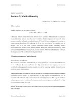
7) Example
The cross-country data for 66 developing countries for 1987 is collected from World Development
Report. The variables are:
Dependent variable: National savings rate (S/Y)
Independent variable: Foreign aid as per cent of GDP (A/Y)



SUMMARY OUTPUT


Regression Statistics
Multiple R 0.570665305
R Square 0.32565889
Adjusted R Square 0.31512231
Standard Error 12.72184023
Observations 66


ANOVA

Df SS MS F Significance F
Regression 1 5002.224173 5002.224 30.90746 5.65198E-07
Residual 64 10358.09401 161.8452
Total 65 15360.31818


Coefficients Standard Error t Stat P-value Lower 95% Upper 95%
Intercept 19.1411184 2.062147087 9.282131 1.82E-13 15.02150973 23.2607271
A/Y -0.872432774 0.156927962 -5.55945 5.65E-07 -1.18593213 -0.55893341
Written by Nguyen Hoang Bao May 20, 2004
Applied Econometrics Simple Linear Regression Model
6



RESIDUAL OUTPUT

Observation Predicted S/Y Residuals
1 8.846411667 -5.846411667
2 9.806087718 0.193912282
… … …
66 19.1411184 5.858881602
Figure 7.1:
Impact of Foreign Aid on National Savings
-80.0
-60.0
-40.0
-20.0
0.0
20.0

40.0
60.0
0.0 10.0 20.0 30.0 40.0 50.0 60.0
Foreign Aid as per cent of GDP
National Savings ratio

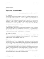
Figure 7.2:
Written by Nguyen Hoang Bao May 20, 2004
Applied Econometrics Simple Linear Regression Model
7
Residual Plot (S/Y-S/Yfit) versus A/Y
-80
-60
-40
-20
0
20
40
0.0 10.0 20.0 30.0 40.0 50.0 60.0
Foreign Aid as per cent of GDP
Residual (e = S/Y-S/Yfit)

8) Functional forms of regression models

We observe that the relationship between Y and X can be nonlinear rather than linear. The functional
form to adopt can often be seen from the data and this is sometimes you should become practiced in.

Semi – logarithmic transformation
Y = β
0

+ β
1
lnX

Y Y






X X


lnY = β
0
+ β
1
X

Y Y





Written by Nguyen Hoang Bao May 20, 2004
Applied Econometrics Simple Linear Regression Model
8

X X


Double – logarithmic transformation
lnY = β
0
+ β
1
lnX

Y Y






X X

Reciprocal Tranformation
Y = β
0
+ β
1
(1/X)

Regressing Y on 1/X allows Y to grow or decline towards a limiting value given by the intercept of
the model.

Y Y

X X


The interpretation of the regression coefficients depends on the functional form adopted.
Specific functional forms Derivatives Interpretation
Constant absolute increment in Y
for one unit change in X
Y = β
0
+ β
1
X
X
Y
β
1
∂
∂
=

Constant absolute increment in Y
for one percent increase in X
Y = β
0

+ β
1
lnX
X/X
Y
β
1
∂
∂
=

Constant rate of growth in Y for
one unit change in X
lnY = β
0
+ β
1
X
X
Y/Y
β
1
∂
∂
=

Written by Nguyen Hoang Bao May 20, 2004
Applied Econometrics Simple Linear Regression Model
9
Constant elasticity (i.e., constant

per cent increase in Y for one per
cent increase in X)
lnY = β
0
+ β
1
lnX
X/X
Y/Y
β
1
∂
∂
=

Constant absolute increment in Y
for one unit change in (1/X)
Y = β
0
+ β
1
(1/X)
X)/1(
Y
β
1
∂
∂
=

If we transform either X or Y, or both, to achieve linearity of the regression line, we should not
forget that, in the process, we also transformed the distribution of Y or X or both. In practice, a
useful rule of thumb is to keep in mind that linear regression tends to work best when both variables
are similarly preferably symmetrically shaped (Hamilton, 1992: 148).

In econometric practice, the logarithmic transformation is very popular. One reason is that functions,
which can be linearised with the aid of logarithms have coefficient which lend themselves to
meaningful economic interpretations, such as elasticity or a growth rate. Another reason is that the
logarithmic transformation frequently, but not always, does the trick with socioeconomic data, which
are often skewed to the right.

References

Bao, Nguyen Hoang (1995), ‘Applied Econometrics’, Lecture notes and Readings,
Vietnam-Netherlands Project for MA Program in Economics of Development.

Hamilton, Lawrence C (1992), Regression with graphics: A Second in Applied Statistics, Pacific
Grove, CA: Brooks Cole.

Maddala, G.S. (1992), ‘Introduction to Econometrics’, Macmillan Publishing Company, New York.

Mukherjee Chandan, Howard White and Marc Wuyts (1998), ‘Econometrics and Data Analysis for
Developing Countries’ published by Routledge, London, UK.
Written by Nguyen Hoang Bao May 20, 2004
Applied Econometrics Simple Linear Regression Model
10
Workshop 2: Simple Regression Models

1) Retrieve data file AIDSAV.WK1, which contains the data for saving rate (S/Y) and the aid ratio

(A/Y).

1.1) Plot the scatter plot of (S/Y) against (A/Y)

S/Y S/YA/Y
), (A/Y –
1.2) Calculate the mean deviations
(S/Y – ); the mean deviations (S/Y– )
2
,
(A/Y–
)
2
; and the product of the mean deviation (S/Y –
S/YA/Y A/Y
)*(A/Y – ).

1.3) Calculate
and from the following regression equation S/Y = + (A/Y)
1β
ˆ
1β
ˆ
0β
ˆ
0β
ˆ

1.4) Calculate the fitted values of S/Y

1.5) Calculate the residual u
i


1.6) Check they sum to zero
∑u
i
= 0

1.7) Calculate the total sum of squares (TSS), the explanatory sum of squares (ESS), and the
residual sum of squares (RSS)

1.8) Calculate the coefficient of determination (R
2
) and correlation coefficient (r)

1.9) Calculate the standard error of the regression (s), the standard error of the slope SE( ), and
the standard error of the intercept SE( )
1β
ˆ
0β
ˆ

1.10) Calculate the t – statistics

1.11) Test the null hypothesis that H
0
: = 0 against ≠ 0. Comment on your results
1β
ˆ

1β
ˆ

1.12) Draw the scatter plot showing the fitted line. Comment on your findings
Written by Nguyen Hoang Bao May 20, 2004
Applied Econometrics Simple Linear Regression Model
11

1.13) Construct 95% confident interval for and
1β
ˆ
0β
ˆ

1.14) Given a specific value of A/Y = 0.12, calculate the prediction interval for S/Y
2) Retrieve data file TOT.WK1, which contains the data for TOT.

2.1) Estimate the following two models
lnTOT = α
0
+ α
1
T
where T = 1, 2, …, 37

lnTOT = β
0
+ β
1
t

where t = 1950, 1951, …, 1986

2.2) What is the relationship between α
0
and β
0
and between α
1
and β
1
. Discuss this
relationship first by looking at your regression results and algebraic demonstration of the
relationship between the coefficients.

3) Draw a scatter plot of consumption against income using the data in data file SRINA.WK1. Plot
on this graph

3.1) the fitted values of consumption from the consumption function

3.2) the upper and lower limits of the confidence interval for the fitted values and discussing on
the shape of the curves you have plotted.

4) Demonstrate algebraically that adding a point (X
n+1
, Y
n+1
) to a sample of n observations will

4.1) not influence the slope coefficient of the regression of Y on X if X
n+1

is equal to sample
mean for X of the n observations

4.2) that the intercept from the regression will probably change even if Y
n+1
is equal to the
sample mean for Y of the n observations

4.3) that if X
n+1
, Y
n+1
lies at the point of means of the sample of observations, then the
regression line is unchanged.
Written by Nguyen Hoang Bao May 20, 2004
Applied Econometrics Simple Linear Regression Model
12

4.4) Generating a numerical data to illustrate your findings



5) Retrieve data file INDO.WK1, which contains the data for income (Y) and expenditure (E= C+I)

5.1) Estimate the following two models:

lnE = α
0
+ α
1

Y
lnE = β
0
+ β
1
lnY

5.2) Draw the scatter plots and the fitted lines on each; one paragraph of discussion.


Written by Nguyen Hoang Bao May 20, 2004