Tài liệu lackwell Publishing, Ltd. Predictors of reproductive cost in female Soay sheep pptx
Bạn đang xem bản rút gọn của tài liệu. Xem và tải ngay bản đầy đủ của tài liệu tại đây (227.67 KB, 13 trang )
Journal of Animal
Ecology
2005
74
, 201–213
© 2005 British
Ecological Society
Blackwell Publishing, Ltd.
Predictors of reproductive cost in female Soay sheep
G. TAVECCHIA*†‡, T. COULSON†#, B. J. T. MORGAN‡, J. M. PEMBERTON§,
J. C. PILKINGTON§, F. M. D. GULLAND¶ and T. H. CLUTTON-BROCK†
†
Department of Zoology, University of Cambridge, Downing Street, Cambridge, CB2 3EJ, UK,
‡
Institute of
Mathematics and Statistics, University of Kent, Canterbury, CT2 7NF, UK,
§
Institute of Cell, Animal and Population
Biology, University of Edinburgh, West Mains Road, Edinburgh EH9 3JT, UK, and
¶
The Marine Mammal Center,
1065 Fort Cronkhite, Sausalito, CA 9496, USA
Summary
1.
We investigate factors influencing the trade-off between survival and reproduction in
female Soay sheep (
Ovis aries
). Multistate capture–recapture models are used to incor-
porate the state-specific recapture probability and to investigate the influence of age and
ecological conditions on the cost of reproduction, defined as the difference between
survival of breeder and non-breeder ewes on a logistic scale.
2.
The cost is identified as a quadratic function of age, being greatest for females breed-
ing at 1 year of age and when more than 7 years old. Costs, however, were only present
during severe environmental conditions (wet and stormy winters occurring when popu-
lation density was high).
3.
Winter severity and population size explain most of the variation in the probability
of breeding for the first time at 1 year of life, but did not affect the subsequent breeding
probability.
4.
The presence of a cost of reproduction was confirmed by an experiment where a
subset of females was prevented from breeding in their first year of life.
5.
Our results suggest that breeding decisions are quality or condition dependent. We
show that the interaction between age and time has a significant effect on variation around
the phenotypic trade-off function: selection against weaker individuals born into cohorts
that experience severe environmental conditions early in life can progressively eliminate
low-quality phenotypes from these cohorts, generating population-level effects.
Key-words
:multistate model, recruitment, survival, trade-off function
Journal of Animal Ecology
(2005)
74
, 201–213
doi: 10.1111/j.1365-2656.2004.00916.x
Introduction
Experimental and correlative studies are increasingly
providing evidence to support theoretical predictions
that reproduction is costly (Clutton-Brock 1984;
Viallefont, Cooke & Lebreton 1995; Berube, Festa-
Bianchet & Jorgenson 1996; Pyle
et al
. 1997; Festa-
Bianchet, Gaillard & Jorgenson 1998; Monaghan, Nager
& Houston 1998; Westendrop & Kirkwood 1998;
Tavecchia
et al
. 2001; Roff, Mostowy & Fairbairn 2002
(Bérubé, Festa-Bianchet & Jorgenson 1999; Festa-
Bianchet
et al
. 1995). In general, this cost is expressed
as a decrease in the future reproductive value through a
decline in (i) survival, (ii) the future probability of
reproduction, and/or (iii) offspring quality (Daan &
Tinbergen 1997). In particular, the presence of a link
between survival and reproduction is a concept under-
pinning the theory of life-history evolution (see Roff
1992; Fox, Roff & Fairbairn 2001). Quantitative stud-
ies of this link allow optimal behaviours and strategies
to be identified as well as possible mechanisms driving
the evolution of life-history tactics (McNamara &
Houston 1996). Although the assumption of a trade-
off between fitness components is implicit in the evo-
lution of life-history tactics, it is not always considered
in models used to explore variation in fitness or popula-
tion growth rate in natural populations (van Tienderen
1995). Rather, a typical approach to explore the effects
of trait variability on population growth rate,
λ
, is to
use perturbation analyses by independently altering
the probability of each fitness component. The covari-
ation between survival and reproduction, however,
*Present address and correspondence: IMEDEA – UIB/
CSIC, C. M. Marques 21, 07190, Esporles, Spain. E-mail:
g.tavecchia.uib.es
#Present address: Department of Biological Sciences, Impe-
rial College at Silwood Park, Ascot, Berks, SL5 7PY, UK
202
G. Tavecchia
et al.
© 2005 British
Ecological Society,
Journal of Animal
Ecology
,
74
,
201–213
is by definition important (Benton & Grant 1999; Caswell
2001). For example, Benton, Grant & Clutton-Brock
1995) developed a stochastic population model of red
deer (
Cervus elaphus
) living on Rum and showed that
stochastic variation in survival or fecundity was never
able to select for an increase in fecundity. If, however,
environmental stochasticity influenced the trade-off
between survival and fecundity,
λ
became more sens-
itive to changes in fecundity. These empirical results are
also supported by theoretical studies showing that a
change in a trade-off function is more effective in pro-
moting life-history diversity than a change in the value
of a single trait (Orzack & Tuljapurkar 2001). Despite
the importance of dynamic modelling of the trade-off
between survival and reproduction (Roff
et al.
2002;
but see Cooch & Ricklefs 1994), empirical evidence is
scarce, with most theoretical studies based on unsup-
ported assumptions about the shape and variation of
the trade-off function (Sibly 1996; Erikstad
et al
. 1998).
There are remarkably few studies where data on sur-
vival and fecundity rates exist over a sufficiently long
period on a suitably large number of animals to allow
detailed examination of the trade-off function (but see
Bérubé, Festa-Bianchet & Jorgenson 1999; Festa-Bianchet
et al
. 1995; Berube, Festa-Bianchet & Jorgenson 1996;
Festa-Bianchet
et al.
1998, where costs of reproduction
in bighorn sheep have been explored). Moreover, the
computation of the trade-off function from long-term
data is complicated by the fact that individuals in nat-
ural populations might breed or die undetected. The
resulting ‘fragmented’ information can generate biases
in estimates of the survival and reproductive rates of
individuals (Nichols
et al
. 1994; Boulinier
et al
. 1997).
Recently developed capture–recapture multistate
models (Arnason 1973; Schwarz, Schweigert & Arnason
1993; Nichols & Kendall 1995) provide a robust ana-
lytical method to model and estimate the reproductive
cost taking into account a detection probability (Nichols
et al
. 1994; Cam
et al
. 1998).
We applied these models to estimate the cost of repro-
duction in the Soay sheep (
Ovis aries
) population living
on the island of Hirta in the St Kilda archipelago (Scot-
land) to investigate factors influencing the shape of the
trade-off function. Previous work on the same population
(Clutton-Brock
et al
. 1996; Marrow
et al
. 1996) has
shown that the optimal reproductive strategy changes
in relation to the phase of population growth, but that
individuals are unable to adjust their effort to the pre-
dicted optima. This inability of females to modify their
strategy to environmental cues was demonstrated by the
fact that the survival of breeding females was lower than
that of non-breeding females in periods of high mortality,
and also varied according to the weight of the individual.
Clutton-Brock
et al
. (1996) considered a model that
incorporated density dependence as an environmental
factor but ignored climatic effects. Recent work, however,
has demonstrated that climatic effects have a substantial
impact on population growth rate (Milner, Elston &
Albon 1999; Catchpole
et al
. 2000; Coulson
et al
. 2001).
Clutton-Brock
et al
. (1996) estimated survival condi-
tionally on animals that were recaptured, which reduced
the amount of data available such that a full investiga-
tion of the effect of the costs of breeding for the most
parsimonious age-structure was not possible. In
addition, Catchpole, Morgan & Coulson (2004) showed
how this kind of conditional inference can give rise to
biased estimates that can lead to flawed conclusions.
In this paper we extend earlier conditional analyses
to investigate further age-dependent costs of reproduc-
tion. We report significant influences of density and cli-
mate on the survival–reproduction trade-off function
while taking into account the probability of recapturing
or re-observing live animals. Correlative studies have
been considered as unlikely systems in which to iden-
tify a trade-off between reproduction and survival (van
Noordwijk & De Jong 1986; Partridge 1992; Reznick
1992) because natural selection is predicted to operate
such that all individuals follow an optimal strategy for
their quality or resource availability. If this were the case,
any trade-off could only be shown by experimentally
preventing individuals from following optimal invest-
ment strategies. In some cases, however, correlative studies
have successfully detected a trade-off (Clutton-Brock
1984; Viallefont
et al
. 1995; Clutton-Brock
et al
. 1996;
Pyle
et al
. 1997; Cam & Monnat 2000; Tavecchia
et al
.
2001). This is presumed to be a consequence of an
individual’s inability to respond to a temporally variable
trade-off function, making the optimum strategy repro-
duction regardless of the cost. As well as reporting
an environmentally determined survival–reproduction
trade-off from the analysis of observational data, we
also present an analysis of an experiment in which a
group of randomly selected female lambs from two
cohorts were artificially prevented from breeding in
their first year of life through progesterone implants.
Methods
Soay sheep are a rare breed thought to be similar to
domestic Neolithic sheep introduced to Britain around
5000
(Clutton-Brock 1999) and to the island of Soay
in the St Kilda archipelago, Scotland, between 0 and
1000
. The studied population was moved to the
island of Hirta in 1932 following voluntary evacuation
of the local human population in 1930, and left un-
managed since. The data analysed in this paper were col-
lected on female Soay sheep marked and recaptured in
the Village Bay area of Hirta from 1986 to 2000. We use
the term ‘recaptured’ to refer to those sheep that were
seen in summer censuses or captured in the August
catch-up, when between 50% and 90% of the sheep liv-
ing in the stud y area are caught. All sheep were initially
captured as lambs within hours of birth and uniquely
marked using plastic ear tags. In successive occasions,
recaptured females were released in two alternative
breeding states: presence or absence of milk when
203
Reproductive cost
in Soay sheep
© 2005 British
Ecological Society,
Journal of Animal
Ecology
,
74
,
201–213
caught in the summer catch-up, or whether they were
with or without lamb when resighted. Data were sorted
in the form of stratified (multistate) encounter-histories
according to the state in which individuals were released.
Arnason (1973) and Schwarz, Schweigert & Arnason
1993), developed a model to estimate the state specific
parameters from this type of data considering the
mutistate capture-histories as the product of three
probabilities: S
x
i
, the probability that an individual in
state x at occasion
i
, is alive at occasion
i
+ 1,
ψ
xy
i
, the
probability conditional on survival that an individual is
in state y at occasion
i
+ 1 having been in state x at occa-
sion
i
, and the state-specific probability of recapture p
x
(see Brownie
et al
. 1993; Nichols & Kendall 1995). In
our case, x and y are N and B, respectively, for the non-
breeding and breeding state. For simplicity, because
only two states are considered,
ψ
xy
is noted
ψ
x
. In model
notation we single out juvenile survival and transition
parameters (age interval from 0 to 1) noted S
′
and
Ψ′
,
respectively. These probabilities do not depend on the
breeding state as ewes start breeding at the earliest at
1 year of age.
Ψ′
is equivalent to the first-year recruitment
probability. Although the date of death was known for
most individuals, we did not integrate recoveries in multi-
state histories as it would generate numerous multiple
additional parameters (see Lebreton, Almeras & Pradel
1999). The date of death, however, was considered in the
conditional analysis of experimental data (see below).
-, -
In a previous analysis of male and female Soay sheep
survival, Catchpole
et al
. (2000) reduced model para-
meters by forming age-classes sharing common survival,
derived from age-dependent estimates of survival prob-
abilities. Subsequently population size and measures
of winter severity were used as covariates within each
sex-by-age group. In the current analysis the model
complexity increases after the incorporation of the
breeding state. As a consequence, the two variables, age
and/or year, had to be further combined or treated as
continuous to reduce the number of possible interactions.
Catchpole
et al
. (2000) and Coulson
et al
. (2001) detailed
the continuous relationship between survival and external
covariates; namely the previous winter population size
(population size, hereafter) and three weather co-
variates: the North Atlantic Oscillation index (NAO
hereafter; Wilby, O’Hare & Barnsley 1997), and February
and March rainfall. When significant, the relationship
between sheep survival and the above covariates was
always negative for all groups. We are interested in
describing the age-specific pattern of the trade-off, so con-
sequently we relied on these previous results to reduce
the number of parameters related to time-dependent
variation by categorizing the 14 yearly intervals of the
study into three groups according to the severity of
environmental conditions. We combined the population
size and NAO (considered a single index of winter
climatic conditions) into a single variable based on their
product moment correlation (
r =
0·032). Along this gradi-
ent we identified three groups based on the values of the
variable (Table 1). These groups correspond roughly to
favourable (negative values;
n
= 4), severe (positive values;
n
= 4) and intermediate environmental conditions (
n
=
6), respectively (Table 1). For age, we considered 10
groups, namely from 0 to 1, from 1 to 2, etc. The last group
included all animals of 9 years or older. The estimate of
breeding cost concerns individuals from 1 to 9 years (9
age classes). In juveniles (from 0 to 1 year), where the
breeding state is not present, we considered a full time
dependence in survival probability (14 levels). A full time
dependence was also assumed for the recapture prob-
ability (Catchpole
et al
. 2000) in addition to a linear effect
of age as suggested by previous analyses (Tavecchia 2000).
To identify the most parsimonious model, we progres-
sively eliminated effects on survival, recapture and
Table 1. NAO index and population size were combined to categorize years into three groups of similar sizes corresponding to
favourable (n = 4), intermediate (n = 6) and severe (n = 4) environmental conditions, respectively (also see text). Note that
intervals are ordered according to the combined variable
Interval
Previous summer
population size
NAO
index
Combined
variable
Environmental
conditions
1995–96 1176 −3·78 −1·807 Favourable
1986–87 710 −0·75 −1·677 Favourable
1990–91 889 1·03 −0·844 Favourable
1987–88 1038 0·72 −0·688 Favourable
1989–90 694 3·96 −0·292 Intermediate
1992–93 957 2·67 −0·239 Intermediate
1999–00 1000 2·8 −0·128 Intermediate
1996–97 1825 −0·2 0·351 Intermediate
1993–94 1283 3·03 0·414 Intermediate
1997–98 1751 0·72 0·503 Intermediate
1991–92 1449 3·28 0·766 Severe
1994–95 1520 3·96 1·089 Severe
1998–99 2022 1·7 1·25 Severe
1988–89 1447 5·08 1·302 Severe
204
G. Tavecchia
et al.
© 2005 British
Ecological Society,
Journal of Animal
Ecology
,
74
,
201–213
transition parameters separately keeping the structure
of other parameters as general as possible (Grosbois &
Tavecchia 2003). For example, if the general model
assumes age-dependent parameters we kept this effect on
survival and recapture when transitions were modelled.
The result of independent step-down selections, on S
′
,
S, p,
Ψ′
and
Ψ
, would be what we term a
consensual
model
including the structure selected in each para-
meter separately. The consensual model would provide a
more parsimonious environment in which to test new
factors or to re-test previously non-significant factors.
This procedure was repeated until no more simplifica-
tion was possible. Models were fitted using the program
MARK1·9 modelling all parameters on a logit scale
(White & Burnham 1998). Model selection was based
on the corrected Akaike’s Information Criterion (AICc;
Burnham & Anderson 1998), providing a compromise
between model deviance and the number of parameters
used (the lowest value of AICc represents the most
parsimonious model). A model selection procedure
following the AICc value inevitably involves an arbitrary
component. For example, Lebreton
et al
. (1992) con-
sidered as equivalent two models with a difference in
AICc of 2. Burnham & Anderson (1998) suggested a
higher threshold of 4 to 7. In this paper we consider
models within 4 AICc values to be equivalent and among
equivalent models we prefer the one with fewest para-
meters. Finally, all structurally estimable parameters
were considered, even if their estimates were close to
the boundaries of the parameter space.
The symbols used in model notation are summarized in
Table 2. Specifically ‘N’ and ‘B’ are subscripts represent
non-breeding and breeding states, respectively; others
symbols are used for factors or covariates and appear
in brackets: ‘y’ represents year as a 14-level factor and
‘e’ represents year as a 3-level factor categorized accord-
ing to environmental conditions; for all parameters, ‘a’
represents age as a 9-level factor; ‘A’ denotes when age
is used as a continuous variable ranging from 1 to 9. A
‘*’ always specifies the statistical interaction between
main effects, a ‘+’ when effects are additive and ‘.’ indi-
cates when no effects are present. Population size is
denoted by ‘P’ and the North Atlantic Oscillation
index by ‘NAO’. In this paper we do not try to model S
B
explicitly. Instead, we shall model S
N
and a measure of
the difference between S
B
and S
N
. Thus, we specifically
denote the cost of reproduction on survival as
∆
S,
defined as:
∆
S = logit(S
N
)
−
logit(S
B
)
We shall adopt linear models for logit(S
N
) and
∆
S, as
functions of covariates. We can see from the above
equation that logit(S
B
) is then also, conveniently, a linear
function of the covariates.
In 1988 and 1990, 37 out of the 154 female lambs released
were treated with a progesterone implant to suppress
oestrus in the following autumn. Implants were made
by mixing 1·5 g powdered progesterone (Sigma P 0130)
with 2·2 g Silastic 382 Medical Grade Elastomer and 1/
3 drop of vulcanizing agent catalyst M (stannous octoate:
Dow Corning, USA). The mix was then extruded into
a plastic mould made from a 2-mL plastic syringe and
the volume adjusted to 2·5 mL. Prior to use, implants
Table 2. Parameters modelled and symbols used in model notation (also see text)
Parameter
S
N
Annual survival probability for an individuals released in the non-breeding state
S
B
Annual survival probability for an individuals released in the breeding state
S′′
′′
Juvenile survival probability (age interval from 0 to 1year)
p
N
The probability of recapture or resight an individual in the non-breeding state
p
B
The probability of recapture or resight an individual in the breeding state
ΨΨ
ΨΨ
N
The probability conditional on survival that an individual leaves the non-breeding state
ΨΨ
ΨΨ
B
The probability conditional on survival that an individual leaves the breeding state
ΨΨ
ΨΨ
′′
′′
Recruitment probability at age 1
∆∆
∆∆
S Cost of reproduction, defined as the difference in state-specific annual survival
∆∆
∆∆
S′′
′′
Cost of reproduction at 1 year old
Effect
a Age (9 levels)
A Age (continuous variable)
y Year (14 levels)
NAO North Atlantic Oscillation index (continuous variable)
P Population size (continuous variable)
e Environmental conditions (3 levels). The 14 yearly intervals are grouped in 3 classes according to the combined
values of the North Atlantic Oscillation index and previous winter population size
* Main effects and their statistical interaction
+ Main effects only (additive effect)
· No effect considered
205
Reproductive cost
in Soay sheep
© 2005 British
Ecological Society,
Journal of Animal
Ecology, 74,
201–213
were soaked in 10% chlorhexidine solution for 20 min
then rinsed in sterile physiological saline. Implants
were implanted subcutaneously in the dorsal midline
following sterile procedures after administration of
3 mL 5% lignocaine to provide local anaesthesia (see
also Heydon 1991 for more details on implants). To
avoid estimating recapture probability when analysing
these data, we restricted the analyses to 140 of the 154
animals whose fate was known because we recovered
the body in the year of death; the year of death of the 14
animals removed from the analysis was unknown (4
were from the treated group). Among the 140 animals
retained for the analysis, 15 had incomplete capture
histories, i.e. they were not captured or seen on one or
more occasions although known to be alive. We relied
on the results of the multistate analysis to ‘complete’
these histories and thus avoided having to model recap-
ture probability explicitly (see Results). In the presence
of a cost of reproduction, treated individuals who
skipped breeding at their first opportunity, at age 1,
should have a higher probability of survival than non-
treated individuals that bred at their first opportunity.
Moreover, if breeding decision is condition dependent,
non-breeding individuals in the untreated group would
be in poorer condition than average. Current reproduc-
tion and the number of previous reproductive events
may have long-term or cumulative costs. In this scenario
treated individuals should exhibit higher survival rates
even after they have started to reproduce.
Results
10
We analysed a total of 2036 observations on 988 differ-
ent females. Model selection started from the general
model given below (Model 1 hereafter):
Model 1 S′(y)S
N
(a
*
e)∆S(a
*
e)/Ψ′(y)Ψ
N
(a
*
e)
Ψ
B
(a
*
e)/p
N
(A + y)/p
B
(A + y)
Model 1 must be viewed as the most general model, i.e.
the one with the largest number of parameters. The
absence of a breeding state in juveniles’ parameters, S′
and Ψ′, allowed us to assume a full year effect, noted ‘y’
(14 levels), and test the influence of external covariates.
The same was not possible for other parameters, which
would depend on environmental conditions (3 levels),
full age, denoted by ‘a’ (9 levels) and state (2 levels,
denoted N and B in subscripts). Ideally we should pro-
vide a goodness-of-fit test of Model 1. Recently Pradel,
Wintrebert & Gimenez (2003) proposed a method to
test the fit of the Arnason–Schwarz model (Schwarz
et al. 1993) in which all parameters are assumed to be
time dependent. This requires the fit of a more general
model in which recaptures depend not only on recap-
ture occasions on the state of arrival, but on the state of
departure as well (see Brownie et al. 1993; Pradel et al.
2003). In our case such a model would have to be fitted
in each cohort separately to account for the age-by-time
interaction. In many cohorts, this resulted in numerical
problems owing to data sparseness and consequently
we were not able to correct for extra-multinomial vari-
ation, should any exist. We began to simplify Model 1 by
eliminating non-significant effects from each parameter
at a time. We confirmed previous findings (Catchpole
et al. 2000) that survival probability changed accord-
ing to age and environmental conditions (Table 3). In
addition, we obtained the first representation of the
full age-dependent pattern of the trade-off function
(Fig. 1a,b). Although breeding state and environmental
conditions significantly influenced survival, the evidence
for variation of the breeding cost was weak at this stage
(Table 3; Fig. 2). Juveniles’ parameters varied signifi-
cantly between years (∆AICc = +262·85 and +63·75,
respectively). In both cases, survival and first-year tran-
sitions, the NAO and the population size, explained a
significant part of the deviance (96% and 72%, respec-
tively), but when a simpler (more constrained) environ-
ment was reached their influence was retained only for
survival (see below). In contrast with previous single-
site analyses, the recapture probability was not influ-
enced by age for either state. A year effect was retained
for non-breeders only (∆AICc = 346·77 − 367·61 =
−20·84, Table 3). Transition probabilities after year 1
were not affected by environmental conditions. An effect
of age, however, was retained for the probability of
breeding after a non-breeding event.
At the end of this first simplification we retained four
consensual models (Table 3) that differ by the presence
of covariates in the probability of recruiting at 1 year
old (Models 2 vs. 4, hereafter) and of age on the breed-
ing cost (Models 3 vs. 5):
Model 2 S′(NAO
*
P)S
N
(a
*
e)∆S(a)/
Ψ′(NAO
*
P)Ψ
N
(a)ΨB(·)/p
N
(y)p
B
(·)
Model 3 S′(NAO
*
P)S
N
(a
*
e)∆S(a)/
Ψ′(y)Ψ
N
(a)Ψ
B
(·)/p
N
(y)p
B
(·)
Model 4 S′(NAO
*
P)S
N
(a
*
e)∆S(·)/
Ψ′(NAO
*
P)Ψ
N
(a)Ψ
B
(·)/p
N
(y)p
B
(·)
and
Model 5 S′(NAO
*
P)S
N
(a
*
e)∆S(·)/Ψ′(y)Ψ
N
(a)Ψ
B
(·)/
p
N
(y)p
B
(·)
As expected, these consensual models including only
the significant effects retained for each parameter led to
a substantial decrease in the AICc value (up to 109·22
points from model 1). Model 3 had the lowest AICc but
model 5 should be preferred for its similar AICc value
and its lower number of parameters (Table 3). Accord-
ing to this model the probability of recapture of non-
breeding ewes increased roughly throughout the study,
ranging from 0·45 in 1987 to 1·00 in 2000. Breeding
ewes were virtually always captured (p
B
= 0·999, 95%
206
G. Tavecchia et al.
© 2005 British
Ecological Society,
Journal of Animal
Ecology, 74,
201–213
confidence limits by profile likelihood: 1·000–0·993
from model 5); this probability is therefore fixed at 1·00
in subsequent models and hereafter for simplicity
omitted from model notation. Model 5 was taken as a
new starting point in the model selection procedure.
This model assumes the survival probability of indi-
viduals of age j in year i to be:
Logit(S
B
ji) = logit(S
N
ji) + γ
where γ is the additive effect of breeding, or ‘the breed-
ing cost’ (∆S). This additive effect could be further
modelled as a quadratic function of age as:
Logit(S
B
ji) = logit(S
N
ji) + (β
0
+ β
1
*
Α + β
2
*
Α
2
)?
where β
0
, β
1
and β
2
are the linear predictors of γ, and A
is the linear age (with 1 < A < 9). This model (Model 6,
hereafter) had a lower AICc value (a decrease of 9·7
points from the consensual model; Table 4). This shows
that reproduction has a negative effect on survival early
and late in life even when the influence of environmental
conditions is accounted for. We investigated whether
the cost was interacting with environmental conditions
by building a model assuming three independent para-
bolas describing the difference in survival between breeders
and non-breeders during severe, intermediate and favour-
able years, respectively (Model 7, hereafter), denoted:
Model 7 S′(NAO
*
P)S
N
(a
*
e)∆S((A + A
2
)
*
e)/
Ψ′(y)Ψ
N
(a)Ψ
B
(·)/p
N
(y)
Table 3. Towards a first consensual model. When one parameter is modelled, the structure of the others is kept general (see text).
The general model (Model 1) is S′(y)S
N
(a
*
e)∆
S
(a
*
e)/Ψ′(y)Ψ
N
(a
*
e)Ψ
B
(a
*
e)/p
N
(A + y)p
B
(A + y). DEV = model deviance,
np = number of structural parameters in the model, AICc = corrected Akaike’s Information Criterion. ∆AICc = difference in
AICc value from the general model. The consensual models are built by considering the structure retained for each parameter
(marked in bold in each case). The model number is in square brackets, i.e. the general model is [1], also see text
Model [model number] np DEV AICc−5000 ∆AICc
Juvenile survival
[1] S′(y) 165 5016·88 367·61 0
S′(NAO
*
P) 155 5028·34 356·58 −11·03
S′(NAO + P) 154 5050·22 376·22 +8·61
S′(·) 153 5304·47 630·46 +262·85
Reproductive cost
[1] S
N
(a
*
e) ∆S(a
*
e) 165 5016·88 367·61 0
S
N
(a
*
e) ∆S(a) 147 5032·73 343·09 −24·52
S
N
(a
*
e) ∆S(·) 139 5052·66 345·25 −22·36
S
N
(a
*
e) ∆S(e) 141 5058·39 355·41 −12·20
S
N
(a
*
e) – 150 5058·18 348·55 −19·06
S
N
(a) ∆S(a) 130 5242·69 515·41 +147·80
Recapture
[1] p
N
(A + y) p
B
(A + y) 165 5016·88 367·61 0
p
N
(y) p
B
(A + y) 164 5019·50 367·98 +0·37
p
N
(A + y) p
B
(·) 151 5029·04 348·32 −19·29
p
N
(y) p
B
(·) 150 5029·72 346·77 −20·84
p
N
(A) p
B
(·) 137 5069·88 358·04 −9·57
p
N
(·) p
B
(·) 136 5078·53 364·48 −3·13
First-year recruitment
[1] Ψ′(y) 165 5016·88 367·60 0
Ψ′(NAO
*
P) 155 5043·05 371·29 +3·68
Ψ′(NAO + P) 154 5043·07 369·06 +1·45
Ψ′(P) 153 5050·83 374·59 +6·98
Ψ′(N) 153 5105·31 429·07 +61·46
Ψ′(·) 152 5109·85 431·36 +63·75
Transitions
[1] Ψ
N
(a
*
e) Ψ
B
(a
*
e) 165 5016·88 367·61 0
Ψ
N
(e) Ψ
B
(a
*
e) 141 5069·85 366·87 −0·74
Ψ
N
(a) Ψ
B
(a
*
e) 147 5042·51 352·86 −14·75
Ψ
N
(·) Ψ
B
(a
*
e) 139 5070·06 362·65 −4·96
Ψ
N
(a
*
e) Ψ
B
(e) 141 5037·85 334·87 −32·74
Ψ
N
(a
*
e) Ψ
B
(a) 147 5036·89 347·25 −20·36
Ψ
N
(a
*
e) Ψ
B
(·) 139 5045·33 337·91 −29·70
Ψ
N
(a) Ψ
B
(e) 123 5056·55 313·92 −53·69
Ψ
N
(a) Ψ
B
(·) 121 5060·63 313·62 −53·99
Consensual models
[2] S′(NAO
*
P)S
N
(a
*
e)∆S(a)/p
N
(y)p
B
(·) /Ψ′(NAO
*
P)Ψ
N
(a)Ψ
B
(·) 68 5124·76 264·19 −103·42
[3] S′(NAO
*
P)S
N
(a
*
e)∆S(a)/ p
N
(y)p
B
(·)/Ψ′(y)Ψ
N
(a)Ψ
B
(·) 79 5095·76 258·39 −109·22
[4] S′(NAO
*
P)S
N
(a
*
e)∆S(·)/p
N
(y)p
B
(·) /Ψ′(NAO
*
P)Ψ
N
(a)Ψ
B
(·) 60 5143·79 266·45 −101·16
[5] S′(NAO
*
P)S
N
(a
*
e)∆S(·)/p
N
(y)p
B
(·) /Ψ′(y)Ψ
N
(a)Ψ
B
(·) 71 5115·21 260·95 −106·66
207
Reproductive cost
in Soay sheep
© 2005 British
Ecological Society,
Journal of Animal
Ecology, 74,
201–213
Model 7 had a lower AICc than the first consensual
model retained (∆AICc =
−
8·9), but some coefficients
had unrealistic values as survival was very close to 1·00
in both states except during severe conditions (Fig. 2).
Model 6 and 7 had similar AICc values. The two mod-
els are describing the data equally well, but for reason
of parsimony, the one assuming an additive effect is
preferred as it has fewer parameters.
At this point we investigated the yearly variation in
reproductive cost for first-year mothers only, for which
the cost appeared to be greatest (Fig. 1b). As with the
juvenile parameters, this restriction allowed us to con-
sider a full year effect and directly test the influence of
covariates. The model with a full year effect on 1-year-
old breeders (noted ) is noted (Model 8, hereafter):
The low AICc value of this model (Table 4) gave a clear
indication of a change in the trade-off value with year
(Fig. 3). Such a year variation could be decomposed
into its components, namely the variation due to a den-
sity-dependent factor (noted P), winter severity (NAO)
and their interaction (P
*
NAO). These covariates
explained 43·3% of the yearly variation (19·3% when
the interaction between the two covariates was not con-
sidered; Table 4). This set of models was built ad hoc to
test the variation in reproductive cost in one particular
age class. They are not based on a priori assumptions
and will not be considered further in the analysis. We
finally reduced the number of parameters of Model 7
by assuming survival to be independent of age in non-
breeding animals. Such an assumption held in inter-
mediate and favourable conditions, but did not in severe
conditions where the effect of age proved to be signi-
ficant regardless of the breeding state (Table 4).
The final model ( Model 9; Tables 4 and 5), was therefore
Model 9 S′(NAO
*
P)S
N
(a
*
e)∆
S
(A + A
2
)/
Ψ′(y)Ψ
N
(A)Ψ
B
(·)/p
N
(y)
According to model 9, the probability of breeding after
a non-breeding event is constant through time but
decreases linearly with the age of the ewe. It is interest-
ing to note that at a population level, old ewes appear
Fig. 1. (a) Age-dependent survival estimates for non-breeding
and breeding ewes ( and ᮀ, respectively) from the model
S′(y)S
N
(a)∆
S
(a)/Ψ′(y)Ψ
N
(a
*
e)Ψ
B
(a
*
e)/p
N
(y + A)p
B
(y + A).
(b) The cost of reproduction expressed as 1 − S
B
/S
N
. In both figures,
bars indicate the 95% confidence interval (by δ-method in b).
Fig. 2. Survival probability for non-breeders () and breeders (ᮀ) according to environmental conditions from the general
model (Model 1). Bars indicate 95% confidence interval (when estimates are 1·00 confidence intervals are not plotted).
′
∆
s
Model 8 S (NAO*P)S (a*e)/
N
′′
′
⋅
∆∆
ΨΨΨ
ss N
NB
yapy
ya
() ()/ ()/
()/ ()/ ()
208
G. Tavecchia et al.
© 2005 British
Ecological Society,
Journal of Animal
Ecology, 74,
201–213
less likely to breed after skipping reproduction the pre-
vious year. The frequency of skipping reproduction
after a breeding event is generally low (0·15), and is not
influenced by environmental conditions or the age of
the ewe (Tables 4 and 5). We obtained further insight
on reproductive investment through the analysis of the
experimental data.
In the two cohorts 1988 and 1990, the proportion of
ewes that survived is markedly different (Fig. 4) as a
result of the interaction between age and environ-
mental conditions on survival probability. Although results
should be treated with caution because of the small
sample sizes, the survival of 1-year-old ewes is lower in
the untreated animals than in the treated ones. In agree-
ment with the correlative analysis, mortality is strongly
associated with breeding (Table 5). However, the survival
Table 4. Towards a final model. The consensual model of Table 3 can be simplified and/or specific effects re-tested in a more
parsimonious environment. Moreover the reproductive trade-off function could be further modelled using a specific function o
f
age. ∆AICc = difference in AICc values from the retained consensual model (Model 5; Table 3). We were not able to further
simplify recapture probabilities. The model number is in square brackets
Model Np DEV AICc−5000 DAICc
Survival and Reproductive cost
[6] S
N
(a
*
e) DS(a
*
e) Y′(y) Y
N
(a) 96 5078·36 277·23 16·37
S
N
(a
*
e) DS(A+A
2
)Y′(y) Y
N
(a) 73 5101·17 251·12 −9·74
[7] S
N
(a
*
e) DS((A + A
2
)
*
e) Y′(y) Y
N
(a) 79 5089·32 251·96 −8·91
S
N
(a
*
e) DS(A + A
2
)
1
Y′(y) Y
N
(a) 73 5106·55 256·50 −4·36
S
N
(a
*
e)
2
DS(·) Y′(y) Y
N
(a) 63 5130·65 259·59 −1·28
S
N
(a
*
e)
3
DS(·) Y′(y) Y
N
(a) 63 5125·61 254·55 −6·32
S
N
(a
*
e)
4
DS(·) Y′(y) Y
N
(a) 63 5147·64 276·58 15·72
S
N
(a
*
e) – Y′(y) Y
N
(a) 70 5121·50 265·12 4·26
S
N
(a
*
e) DS(e) Y′(y) Y
N
(a) 73 5112·34 262·29 1·43
[8] S
N
(a
*
e) DS′(y)DS(·) Y′(y) Y
N
(a) 83 5071·30 242·42 −18·44
S
N
(a
*
e) DS′(NAO
*
P)DS(·) Y′(y) Y
N
(a) 74 5092·24 244·30 −16·56
S
N
(a
*
e) DS′(NAO + P)DS(·) Y′(y) Y
N
(a) 73 5101·09 251·04 −9·82
S
N
(a
*
e) DS′(NAO)DS(·) Y′(y) Y
N
(a) 72 5106·32 254·17 −6·70
S
N
(a
*
e) DS′(P)DS(·) Y′(y) Y
N
(a) 72 5106·50 254·35 −6·51
S
N
(a
*
e) DS′(·)DS(·) Y′(y) Y
N
(a) 71 5108·21 253·94 −6·92
Transitions
S
N
(a
*
e) DS(·) Y′(y) Y
N
(A) 64 5122·50 253·53 −7·33
S
N
(a
*
e) DS(·) Y′(y) Y
N
(·) 63 5137·57 266·51 5·65
Final model
[9] S
N
(a
*
e)
5
DS(A + A
2
)Y′(y) Y
N
(A) 50 5128·37 230·22 −30·65
1
Breeding cost is a function of age during severe conditions only.
2
Non-breeders’ survival is constant during favourable conditions.
3
Non-breeders’ survival is constant during intermediate conditions.
4
Non-breeders’ survival is constant during severe conditions.
5
Non-breeders’ survival is constant during intermediate and favourable conditions.
Fig. 3. Yearly variation in the reproductive cost, expressed as
1 − S
B
/S
N
, of first year old ewes from Model 6. Years are ordered
from left to right according to increasing values of the variable
combining NAO and population size. High values correspond to
severe ecological conditions. The solid line represents the trend.
This relationship remains positive even when 1994 and/or 1988
are eliminated. Note that the maximum value of the y-axis is 0·8.
Fig. 4. Proportion of ewes alive according to age, cohort
(dashed lines = 1988; solid lines = 1990) and treatment (solid
symbols = treated; open symbols = untreated).
209
Reproductive cost
in Soay sheep
© 2005 British
Ecological Society,
Journal of Animal
Ecology, 74,
201–213
of treated animals is also higher than survival of non-
breeding untreated animals in both cohorts. This is
what we expected if breeding decisions depended on
individual quality or condition. In adults, for example
aged 5 years, a breeding cost was virtually absent regard-
less of the treatment group or the cohort. The propor-
tion of breeding ewes in this age class was high (Table 5)
suggesting that most animals were of good quality or in
good body condition. Our previous results (see above
and Fig. 2) suggest that breeding is costly for old ani-
mals as well as for 1-year-old ewes. This is supported
experimentally only for ewes born in 1988.
Discussion
Previous evidence of a survival cost of reproduction in
female Soay sheep came from the conditional analyses
in Clutton-Brock et al. (1996) and Marrow et al. (1996).
By directly modelling the variation in the trade-off
function in a capture–recapture framework we have
extended their results showing: (i) that the cost of
reproduction varies as a quadratic function of the age
of the mother, (ii) that it changes with both density-
dependent and density-independent factors and their
interaction, (iii) that these have no effect on the prob-
ability of changing reproductive state, (iv) that repro-
duction is condition-dependent, and (v) that an early
cost of reproduction might have a key role in the selec-
tion of high quality phenotypes within cohorts. Our
results should be considered in comparison to work on
wild bighorn sheep living in Alberta, Canada, where costs
of reproduction have been shown to be age- and mass-
dependent and associated with density (Festa-Bianchet
et al. 1998), as well as previous reproductive history
(Bérubé et al. 1996). This is the only other detailed study
of wild sheep we are aware of that permits estimates of
factors influencing the costs of reproduction. Our results
show considerable similarity with the bighorn sheep
work, suggesting that the costs of reproduction may
typically be age-dependent and associated with envi-
ronmental variation in large mammals. There is also a
literature detailing the costs of reproduction in domestic
sheep (e.g. Mysterud et al. 2002) but given the obvious
differences between the ecology of domestic and wild
sheep we do not discuss this in any further detail.
Correlative studies are not expected to identify a trade-
off between reproduction and survival (van Noordwijk
& De Jong 1986; Partridge 1992; Reznick 1992) because
natural selection is predicted to operate such that all
individuals follow an optimal strategy based on their
quality or on resource availability (van Noordwijk, van
Balen & Scha rloo 1981). When a trade-off is fluctuating
in response to unpredictable environmental variation,
however, the optimum strategy could be to reproduce
regardless of the cost (Benton et al. 1995) and correla-
tive studies could prove useful (Clutton-Brock 1984;
Viallefont et al. 1995; Clutton-Brock et al. 1996; Pyle
et al. 1997; Cam & Monnat 2000; Tavecchia et al. 2000).
In our case, density and climate predicted reproductive
cost: these covariates explained one third of the variation
in reproductive cost in 1-year-old ewes, mainly through
their interaction. Given such uncertainty, the payoff of
a constant level of investment is probably greater than the
payoff obtained by not breeding (Marrow et al. 1996). A
fluctuating trade-off has also been found in Soay sheep
rams (Stevenson & Bancroft 1995; Jewell 1997) that exhibit
a cost of reproduction associated with male-male
conflicts during the rut. Stevenson & Bancroft (1995)
experimentally proved that early reproduction carries a
survival cost in young male when population density is
Table 5. Survival and breeding proportions of treated and untreated females from the 1988 and 1990 cohorts. Values for
individuals that survived until age 5 and = 9 are reported as well. – denotes non-estimable
Cohort
1988 1990
Treated (n = 20) Untreated (n = 59) Treated (n = 13) Untreated(n = 48)
Age 1
Breeding proportion – 0·20 – 0·69
Breeding cost – 0·43 – 0·27
Mortality of non breeders 0·00 0·13 0·10 0·15
Mortality of breeders – 0·50 – 0·38
Age 5
Breeding proportion 0·40 1·00 0·80 0·75
Breeding cost 0·00 0·00 0·00 0·00
Mortality of non breeders 0·00 0·00 0·00 0·00
Mortality of breeders 0·00 0·00 0·00 0·00
Age = 9
Breeding proportion 0·40 0·80 0·50 0·56
Breeding cost 0·50 0·25 0·00 0·00
Mortality of non breeders 0·00 0·00 0·00 0·00
Mortality of breeders 0·50 0·25 0·00 0·00
210
G. Tavecchia et al.
© 2005 British
Ecological Society,
Journal of Animal
Ecology, 74,
201–213
high. Despite this, precocial mating is favoured owing
to the high success achieved in particular years of the
population cycle (Stevenson & Bancroft 1995). The low
frequency of severe conditions prevents a high payoff
for those individuals that skip reproduction early in life.
The reproductive cost varied as a quadratic function of
age, being higher in young and old age classes but absent
between 3 and 7 years (Fig. 1b). This pattern is common
to other large herbivores: Mysterud et al. (2002) con-
cluded that the early onset of reproductive senescence
in domestic sheep may be because of a trade-off between
breeding events and litter size. An age-dependent cost of
reproduction could also be a characteristic of other long-
lived animals. For example, a greater cost of reproduction
at a young age has been found in red deer (Cervus elaphus)
(Clutton-Brock 1984), Californian gulls (Larus clifor-
nianus) (Pyle et al. 1997), lesser snow geese (Anas caer-
ulescens caerulescens) (Viallefont et al. 1995) and greater
flamingos (Phenicopterus ruber roseus) (Tavecchia et al.
2001; but see McElligot, Altwegg & Hayden. 2002).
The association between age and the cost of repro-
duction could be because of natural selection progres-
sively removes low-quality phenotypes. Results from
experimental data suggest that breeding-induced mor-
tality might act as a filter selecting against low-quality
phenotypes. On average, juveniles prevented from breed-
ing in a severe year (cohort 1988) are also less likely to
breed later in life than untreated juveniles; however,
this was not the case for juveniles born in 1990. One
possible explanation is that low-quality individuals in
the treated group were not selected against early in life.
Alternatively, the effect of implants persisted beyond
the first year for the 1988 cohort, but not for the 1990
cohort. Our data set is too small to distinguish between
these two hypotheses. Further support for the selection
hypothesis, however, comes from the survival analysis
conditional on animals known to be dead, of the 1986–
92 cohorts (Fig. 5) in which adult mortality is depressed
in cohorts that experienced severe conditions early in
life. The selection hypothesis, however, does not explain
why the cost of reproduction re-appears in old age classes.
This result provides either evidence for senescence in
breeding performance or of a greater investment in
reproduction by those animals with lower reproductive
values. The senescence-hypothesis is supported by the
fact that the probability of breeding after a non-breeding
event is low in older animals. A similar result was found
in male fallow deer (Dama dama) for which reproduc-
tion probability declines with age despite an apparent
absence of cost of reproduction (McElligot et al. 2002).
‒
Long-term individual-based information is often in-
complete because animals might breed or die undetected
and unbiased estimates can only be obtained by fitting
models that include a recapture probability (Burnham
et al. 1987; Lebreton et al. 1992). The number of para-
meters generated by these models dramatically increases
with the number of states, providing limited power to
test specific hypotheses with most ecological data sets
(Tavecchia et al. 2001; Grosbois & Tavecchia 2003).
Moreover, in models with large numbers of parameters,
the likelihood function can encounter convergence prob-
lems, especially when estimates are near the 0–1 bound-
aries (see Results). These complications have probably
contributed to the relative unpopularity of multistate
models (Clobert 1995). In some cases researchers pre-
fer to assume a recapture probability of 1·00 and risk
biasing estimates. The magnitude of biases in para-
meter estimates depends on the study system (Boulinier
et al. 1997). For example, the recapture probability of
female Soay sheep was high but the assumption of a
recapture probability equal to, or very close to, 1·00
only held for breeding females. In this case, avoiding a
capture–recapture framework would have led to an
overestimate of the breeding proportion and an under-
estimate of state specific survival probabilities. Recapture
probabilities should be interpreted in both a biological
Fig. 5. Proportion of female sheep alive according to age and cohort.
211
Reproductive cost
in Soay sheep
© 2005 British
Ecological Society,
Journal of Animal
Ecology, 74,
201–213
and statistical setting. For example when observations
are made during the reproductive period, the age-
specific probabilities of recapture could provide insights
on the recruitment probability (Clobert et al. 1994) and
the pattern of reproductive skipping (Pugesek & Diem
1990; Pugesek et al. 1995; Viallefont et al. 1995). In our
case, an important result was that breeding females were
virtually always captured or resighted. As a consequence,
when analysing the experimental data, we were able to
make the assumption that all individuals known to be
alive that escaped recapture were in a non-breeding state.
The analyses we report here suffer from two obvious
limitations. First, although body condition is known to
play an important role in breeding decisions (Marrow
et al. 1996; Andersen et al. 2000), continuous time-
varying covariates like weight cannot be used as predictors
in a capture–recapture framework (Nichols & Kendall
1995). Moreover, individual-level processes, like ex-
perience, can also be important but cannot currently be
modelled in a multistate mark–recapture framework
(see Cam & Monnat 2000). A second limitation of our
approach is that recoveries – information on animals
found dead – cannot be included in analyses. This at
first seems an important weakness of a method with the
ultimate aim of estimating mortality. However, when
capture probability is high, as in our case, the estimates
provided by analysing recaptures alone can be expected
to produce precise estimates; adding recovery information
will not appreciably alter conclusions. Despite these
limitations, the advantage is that recruitment, proba-
bility of reproductive skipping, state-specific survival and
recapture probabilities have been modelled and estimated
simultaneously (Table 6).
Conclusions
For any given trait, optimality theory predicts that
evolution should select for the value that maximizes
fitness. Spatial and temporal variability in selection
pressures can generate variation in the optimum trait
value and lead to multiple life-history tactics within
a single population or among populations (Daan &
Tinbergen 1997; but see Cooch & Ricklefs 1994). Recent
work has shown that a change in the trade-off function
is more effective in promoting life-history diversity
between and within populations than a change in the
value of a single trait (Orzack & Tuljapurkar 2001; Roff
et al. 2002) and that more attention should be focused
on variation around the trade-off function. Multistate
models offer the ideal framework to address these
questions in natural populations. Our analysis showed
that breeding is costly and that this cost changes with
age and environmental conditions. A trade-off between
survival and reproduction is generally expected if indi-
viduals behave in a maladaptive way. Alternatively,
Clutton-Brock et al. (1996) concluded that the optimal
strategy is to breed regardless of the cost, given that
animals are not able to predict variation in mortality
(see also Marrow et al. 1996). Our results confirmed
the latter hypothesis, but demonstrated that both
density-dependent and independent factors need to be
considered when modelling reproductive tactics. Fur-
ther work on the Soay sheep should focus on the ana-
lysis of mortality during different stages of the breeding
cycle using post mortem information. It should, however,
be noted that the current results reflect the ‘average’
value of the age-specific reproductive tactics. This does
not necessarily mean that all individuals exhibit an
‘average’ strategy. Further work should focus on parental
investment conditional to breeding decisions and on the
relative cost of the different stages of the breeding cycle.
Acknowledgements
We thank Tony Robinson, Adrew MacColl and many
volunteers involved in the Soay Sheep project who
Table 6. Predictors of survival, recapture, cost of reproduction and recruitment at 1 year in female Soay sheep. Estimates of linear
regression parameters are from the retained model. Notation as in Table 1 except ‘^’ which denotes firs order interaction between
main effects in the regression
Parameter Predictors Effect
Juvenile survival Population size and NAO Logit(S′) = 0·56 – 0·31(P) – 1·44(NAO) – 0·71(NAO^P)
Adult survival Environmental conditions Lower during severe environmental conditions
During severe conditions only (9 levels)
Age
Cost of reproduction Environmental conditions Higher during severe conditions only
Mother age Logit(S
B
) = logit(S
N
) – 1.56 + 0.85(A) – 0.09(A
2
)
Recruitment probability at 1-year old Time Yearly variation mainly explained by the NAO
and the P as:
Logit(Y′) = −0·47 – 0·24(P) – 1·30(NAO) – 0·07(NAO^P)
but not retained as the only predictors
Probability of breeding after a
non-breeding event
Age Logit(Y
N
) = 0·38 – 0·14(A)
Probability of non-breeding
after a breeding event
–Y
B
= 0·15
Probability of recapture Time In non-breeders only
Breeding state p
B
=1·00
212
G. Tavecchia et al.
© 2005 British
Ecological Society,
Journal of Animal
Ecology, 74,
201–213
helped to collect the data throughout the study. Many
thanks to F. Sergio and Ken Wilson who commented
on an early version of the manuscript and to Andrew
Loudon for manufacturing the progesterone implants.
M. Festa-Bianchet provided useful comments. We thank
the National Trust for Scotland and the Scottish
Natural Heritage for permission to work on St Kilda,
and the Royal Artillery for logistical support, NERC and
the Wellcome Trust for providing financial support.
G.T. was supported by a BBRSC grant (ref. 96/E14253).
References
Andersen, R., Gaillard, J M., Linell, J.D. & Duncan, P. (2000)
Factors affecting maternal care in an income breeder, the
European roe deer. Journal of Animal Ecology, 69, 1–12.
Arnason, A.N. (1973) The estimation of population size,
migration rates and survival in a stratified population.
Research on Population Ecology, 15, 1–8.
Benton, T.G. & Grant, A. (1999) Elasticity analysis as an
important tool in evolutionary and population ecology.
Trend in Ecology and Evolution, 14, 467–471.
Benton, T.G., Grant, A. & Clutton-Brock, T.H. (1995) Does
environmental stachasticity matter? Analysis of red deer
life-history on Rum. Evolutionary Ecology, 9, 559–574.
Bérubé, C.H., Festa-Bianchet, M. & Jorgenson, J.T. (1996)
Reproductive costs of sons and daughters in Rocky Mountain
bighorn sheep. Behavioral Ecology, 7, 60–68. 20.
Bérubé, C., Festa-Bianchet, M. & Jorgenson, J.T. (1999) Indi-
vidual differences, longevity, and reproductive senescence
in bighorn ewes. Ecology, 80, 2555–2565.
Boulinier, T., Sorci, G., Clobert, J. & Danchin, E. (1997) An
experimental study of the costs of reproduction in the Kit-
tiwake Rissa tridactyla: comment. Ecology, 78, 1284–1287.
Brownie, C., Hines, J.E., Nichols, J.D., Pollock, K.H. &
Hestbeck, J.B. (1993) Capture–recapture studies for multiple
stata including non-markovian transitions. Biometrics, 49,
1173–1187.
Burnham, K.P. & Anderson, D.R. (1998) Model Selection and
Inference. A Practical Information – Theoretical Approach.
Springer-Verlag, New York.
Burnham, K.P., Anderson, D.R., White, G.C., Brownie, C. &
Pollock, K.H. (1987) Design and Analysis Methods for Fish
Survival Experiments Based on Release-Recapture. Amer-
ican Fisheries Society, Bethesda, Maryland.
Cam, E., Hines, J.E., Monnat, J Y., Nichols, J.D. & Danchin, E.
(1998) Are adult non-breeders prudent parents? The kitti-
wake model. Ecology, 79, 2917–2930.
Cam, E. & Monnat, J Y. (2000) Apparent inferiority of first-time
breeders in the kittiwake: the role of heterogeneity among
age classes. Journal of Animal Ecology, 69, 380–394.
Caswell, H. (2001) Matrix Population Models, 2nd edn.
Sinauer Press, Sunderland, Massachusetts, USA.
Catchpole, C.K., Morgan, B.J.T. & Coulson, T.N. (2004)
Conditional methodology for individual case-history data.
Applied Statistics, 53, 1, 123–131.
Catchpole, C.K., Morgan, B.J.T., Coulson, J.N., Freeman,
S.N. & Albon, S.D. (2000) Factors influencing Soay sheep
survival. Journal of Applied Statistics, 49, 453–472.
Clobert, J. (1995) Capture–recapture and evolutionary biology:
a difficult wedding. Journal of Applied Statistics, 22, 989–1008.
Clobert, J., Lebreton, J D., Allainé, D. & Gaillard, J M.
(1994) The estimation of age-specific breeding probabilities
from capture or resightings in vertebrate populations II.
Longitudinal models. Biometrics, 50, 375–387.
Clutton-Brock, T.H. (1984) Reproductive effort and terminal
investment. American Naturalist, 123, 212–229.
Clutton-Brock, J. (1999) The Natural History of Domesticated
Mammals, 2nd edn. Cambridge University Press, Cambridge.
Clutton-Brock, T.H., Stevenson, I.R., Marrow, P., MacColl,
A.D., Houston, A.I. & McNamara, J.M. (1996) Population
fluctuations, reproductive costs and life-history tactics in female
Soay sheep. Journal of Animal Ecology, 65, 675–689.
Cooch, E.G. & Ricklefs, R.E. (1994) Do variable environ-
ments significantly influence optimal reproductive effort in
birds? Oikos, 69, 447–459.
Coulson, T., Catchpole, E.A., Albon, S.D., Morgan, B.J.T.,
Pemberton, J.M., Clutton-Brock, T.H., Crawley, M.J. &
Grenfell, B.T. (2001) Age, sex, density, winter weather and
population crashes in Soay sheep. Science, 292, 1528–1531.
Daan, S. & Tinbergen, J.M. (1997) Adaptation of life histories.
Behavioural Ecology: An Evolutionary Approach (eds Krebs,
J.R. & Davies, N.B.), pp. 311–333. Blackwell, Oxford.
Erikstad, K.E., Fauchald, P., Tveraa, T. & Steen, H. (1998) On
the cost of reproduction in long-lived birds: the influence of
environmental variability. Ecology, 79, 1781–1788.
Festa-Bianchet, M., Gaillard, J.M. & Jorgenson, J.T. (1998)
Mass- and density-dependent reproductive success and
reproductive costs in a capital breeder. American Naturalist,
152, 367–379.
Festa-Bianchet, M., Jorgenson, J.T., Lucherini, M. &
Wishart, W.D. (1995) Life history consequences of variation
in age of primiparity in bighorn ewes. Ecology, 76, 871–
881.
Fox, C.W., Roff, D.A. & Fairbairn, D.J. (2001) Evolutionary
Ecology. Concepts and Case Studies, 22. Oxford University
Press, Oxford.
Grosbois, V. & Tavecchia, G. (2003) A new way of modelling
dispersal with capture–recapture data: disentangling
decision of leaving and settlement. Ecology, 84, 1225–
1236.
Heydon, M.J. (1991) The control of seasonal changes in repro-
duction and food intake in grazing red deer hinds Cervus
elaphus. PhD Thesis. University College, London.
Jewell, P.A. (1997) Survival and behaviour of castrated Soay
sheep Ovis aries in a feral island population on Hirta, St.
Kilda, Scotland. Journal of Zoology, 243, 623–636.
Lebreton, J D., Almeras, T. & Pradel, R. (1999) Competing
events, mixtures of information and multistrata recapture
models. Bird Study (46 Suppl.), 39–46.
Lebreton, J.D., Burnham, K.P., Clobert, J. & Anderson, D.R.
(1992) Modeling survival and testing biological hypotheses
using marked animals: a unified approach with case studies.
Ecological Monographs, 62, 67–118.
Marrow, P., McNamara, J.M., Houston, A.I., Stevenson, I.R.
& Clutton-Brock, T.H. (1996) State-dependent life history
evolution in Soay sheep: dynamic modelling of reproductive
scheduling. Philosophical Transaction of the Royal Society
of London Series B, 351, 17–32.
McElligot, A.G., Altwegg, R. & Hayden, T.J. (2002) Age-
specific survival and reproductive probabilities: evidence for
senescence in male fallow deer (Dama dama). Proceeding of
the Royal Society of London Series B, 269, 1129–1137.
McNamara, J.M. & Houston, A.I. (1996) State-dependent
life-history. Nature, 380, 215–221.
Milner, J.M., Elston, D.A. & Albon, S.D. (1999) Estimating
the contributions of population density and climatic fluc-
tuations to interannual variation in survival of Soay sheep.
Journal of Animal Ecology, 68, 1235–1247.
Monaghan, P., Nager, R.G. & Houston, D.C. (1998) The price
of eggs: increased investment in egg production reduces the
offspring rearing capacity of parents. Proceeding of the
Royal Society of London. Series B, 265, 1731–1735.
Mysterud, A., Steinheim, G., Yoccoz, N.G., Holand, O. &
Stenseth, N.C. (2002) Early onset of reproductive senescence
in domestic sheep, Ovis aries. Oikos, 97, 177–183.
Nichols, J.D., Hines, J.E., Pollock, K.H., Hinz, R.L. & Link,
W.A. (1994) Estimating breeding proportions and testing
hypotheses about costs of reproduction with capture–
recapture data. Ecology, 75, 2052–2065.
213
Reproductive cost
in Soay sheep
© 2005 British
Ecological Society,
Journal of Animal
Ecology, 74,
201–213
Nichols, J.D. & Kendall, W.L. (1995) The use of multi-state
capture–recapture models to address questions in evolu-
tionary ecology. Journal of Applied Statistics, 22, 835–846.
van Noordwijk, A.J. & De Jong, G. (1986) Acquisition and
allocation of resources: their influence on variation in life-
history tactics. American Naturalist, 128, 137–142.
van Noordwijk, A.J., van Balen, J.H. & Scharloo, W. (1981)
Genetic and environmental variation in clutch size of the
great tit. Netherland Journal of Zoology, 31, 342–372.
Orzack, S.H. & Tuljapurkar, S. (2001) Reproductive effort in
variable environments, or environmental variation is for the
birds. Ecology, 82, 2659–2665.
Partridge, L. (1992) Measuring reproductives costs. Trends in
Ecology and Evolution, 7, 99–100.
Pradel, R., Wintrebert, C.L.M. & Gimenez, O. (2003) A
proposal for a goodness-of-fit test to the Arnason-
Schwarz multisite capture–recapture model. Biometrics,
59, 43–53.
Pugesek, B.H. & Diem, K.L. (1990) The relationship between
reproduction and survival in known-aged California gulls.
Ecology, 71, 811–817.
Pugesek, B.H., Nations, C., Diem, K.L. & Pradel, R. (1995)
Mark-resighting analysis of California gull population.
Journal of Applied Statistics, 22, 625–639.
Pyle, P., Nur, N., Sydeman, J. & Emslie, D. (1997) Cost of
reproduction and the evolution of deferred breeding in the
wester gull. Behavioral Ecology, 8, 140–147.
Reznick, D. (1992) Measuring the costs of reproduction.
Trends in Ecology and Evolution, 7, 42–45.
Roff, D.A. (1992) The Evolution of Life Histories. Theory and
Analysis. Chapman & Hall, New York. 24.
Roff, D.A., Mostowy, S. & Fairbairn, D.J. (2002) The evo-
lution of trade-offs: testing predictions on response to
selection and environmental variation. Evolution, 56, 84–95.
Schwarz, C.J., Schweigert, J.F. & Arnason, A.N. (1993) Esti-
mating migration rates using tag- recovery data. Biomet-
rics, 49, 177–193.
Sibly, R.M. (1996) Life history evolution in heterogeneous
environments: a review of theory. Philosophical Transactions
of the Royal Society of London Series B, 351, 1349–1359.
Stevenson, I.R. & Bancroft, D.R. (1995) Fluctuating trade-
offs favour precocial maturity in male Soay sheep. Proceed-
ings of the Royal Society of London Series B, 262, 267–275.
Tavecchia, G. (2000) Female Soay Sheep Survival from 1986 to 2000.
Unpublished report 2002. . cam.ac.uk/
ZOOSTAFF/larg/pages/anal86.pdf.
Tavecchia, G., Pradel, R., Boy, V., Johnson, A. & Cézilly, F.
(2001) Sex- and age-related variation in survival probability
and the cost of the first reproduction in breeding Greater
Flamingos. Ecology, 82, 165–174.
van Tienderen, P.H. (1995) Life cycle trade-offs in matrix
population model. Ecology, 76, 2482–2489.
Viallefont, A., Cooke, F. & Lebreton, J D. (1995) Age-specific
costs of first-time breeding. Auk, 112, 67–76.
Westendrop, R.G.J. & Kirkwood, T.B.L. (1998) Human longevity
and the cost of reproductive success. Nature, 396, 743–746.
White, G.C. & Burnham, K.P. (1999) Program MARK:
survival estimation from populations of marked animals.
Bird Study, 46 (Suppl.), 120–129.
Wilby, R.L., O’Hare, G. & Barnsley, N. (1997) The North
Altantic Oscillation Index and British Isles climate vari-
ability. Weather, 52, 266–276.
Received 17 March 2004; revision received 12 May 2004