Tài liệu Đề tài " Geometry of the uniform spanning forest: Transitions in dimensions 4, 8, 12, . . . " pptx
Bạn đang xem bản rút gọn của tài liệu. Xem và tải ngay bản đầy đủ của tài liệu tại đây (568.53 KB, 28 trang )
Annals of Mathematics
Geometry of the uniform
spanning forest: Transitions
in dimensions 4, 8, 12, . . .
By Itai Benjamini, Harry Kesten, Yuval Peres, and
Oded Schramm
Annals of Mathematics, 160 (2004), 465–491
Geometry of the uniform spanning forest:
Transitions in dimensions 4, 8, 12,
By Itai Benjamini, Harry Kesten, Yuval Peres, and Oded Schramm*
Abstract
The uniform spanning forest (USF) in Z
d
is the weak limit of random,
uniformly chosen, spanning trees in [−n, n]
d
. Pemantle [11] proved that the
USF consists a.s. of a single tree if and only if d ≤ 4. We prove that any two
components of the USF in Z
d
are adjacent a.s. if 5 ≤ d ≤ 8, but not if d ≥ 9.
More generally, let N (x, y) be the minimum number of edges outside the USF
in a path joining x and y in Z
d
. Then
max
N(x, y): x, y ∈ Z
d
=
(d − 1)/4
a.s.
The notion of stochastic dimension for random relations in the lattice is intro-
duced and used in the proof.
1. Introduction
A uniform spanning tree (UST) in a finite graph is a subgraph chosen
uniformly at random among all spanning trees. (A spanning tree is a subgraph
such that every pair of vertices in the original graph are joined by a unique
simple path in the subgraph.) The uniform spanning forest (USF) in Z
d
is
a random subgraph of Z
d
, that was defined by Pemantle [11] (following a
suggestion of R. Lyons), as follows: The USF is the weak limit of uniform
spanning trees in larger and larger finite boxes. Pemantle showed that the
limit exists, that it does not depend on the sequence of boxes, and that every
connected component of the USF is an infinite tree. See Benjamini, Lyons,
Peres and Schramm [2] (denoted BLPS below) for a thorough study of the
construction and properties of the USF, as well as references to other works on
the subject. Let T (x) denote the tree in the USF which contains the vertex x.
*Research partially supported by NSF grants DMS-9625458 (Kesten) and DMS-9803597
(Peres), and by a Schonbrunn Visiting Professorship (Kesten).
Key words and phrases. Stochastic dimension, Uniform spanning forest.
466 ITAI BENJAMINI, HARRY KESTEN, YUVAL PERES, AND ODED SCHRAMM
Also define
N(x, y) = min
number of edges outside the USF in a path from x to y
(the minimum here is over all paths in Z
d
from x to y).
Pemantle [11] proved that for d ≤ 4, almost surely T (x)=T(y) for all
x, y ∈ Z
d
, and for d>4, almost surely max
x,y
N(x, y) > 0. The following
theorem shows that a.s. max N (x, y) ≤ 1 for d =5, 6, 7, 8, and that max N (x, y)
increases by 1 whenever the dimension d increases by 4.
Theorem 1.1.
max
N(x, y): x, y ∈ Z
d
=
d − 1
4
a.s.
Moreover, a.s. on the event
T (x) = T (y)
, there exist infinitely many disjoint
simple paths in Z
d
which connect T (x) and T(y) and which contain at most
(d − 1)/4 edges outside the USF.
It is also natural to study
D(x, y) := lim
n→∞
inf{|u − v| : u ∈ T (x),v ∈ T (y), |u|, |v|≥n},
where |u| = u
1
is the l
1
norm of u. The following result is a consequence of
Pemantle [11] and our proof of Theorem 1.1.
Theorem 1.2. Almost surely, for all x, y ∈ Z
d
,
D(x, y)=
0 if d ≤ 4,
1 if 5 ≤ d ≤ 8 and T (x) = T (y),
∞ if d ≥ 9 and T (x) = T (y).
When 5 ≤ d ≤ 8, this provides a natural example of a translation invariant
random partition of Z
d
, into infinitely many components, each pair of which
comes infinitely often within unit distance from each other.
The lower bounds on N(x, y) follow readily from standard random walk
estimates (see Section 5), so the bulk of our work will be devoted to the upper
bounds.
Part of our motivation comes from the conjecture of Newman and Stein
[10] that invasion percolation clusters in Z
d
, d ≥ 6, are in some sense
4-dimensional and that two such clusters, which are formed by starting at
two different vertices, will intersect with probability 1 if d<8, but not if
d>8. A similar phenomenon is expected for minimal spanning trees on the
points of a homogeneous Poisson process in R
d
. These problems are still open,
as the tools presently available to analyze invasion percolation and minimal
GEOMETRY OF THE UNIFORM SPANNING FOREST
467
spanning forests are not as sharp as those available for the uniform spanning
forest.
In the next section the notion of stochastic dimension is introduced. A
random relation R⊂Z
d
× Z
d
has stochastic dimension d − α, if there is some
constant c>0 such that for all x = z in Z
d
,
c
−1
|x − z|
−α
≤ P[xRz] ≤ c|x − z|
−α
,
and if a natural correlation inequality (2.2) (an upper bound for P[xRz, yRw])
holds. The results regarding stochastic dimension are formulated and proved
in this generality, to allow for future applications.
The bulk of the paper is devoted to the proof of the upper bound on
max N(x, y) in (1.1). We now present an overview of this proof. Let U
(n)
be
the relation N(x, y) ≤ n − 1. Then xU
(1)
y means that x and y are in the same
USF tree, and xU
(2)
y means that T (x) is equal to or adjacent to T (y). We
show that U
(1)
has stochastic dimension 4 when d ≥ 4. When R, L⊂Z
d
× Z
d
are independent relations with stochastic dimensions dim
S
(R) and dim
S
(L),
respectively, it is proven that the composition LR (defined by xLRy if and only
if there is a z such that xLz and zRy) has stochastic dimension min{dim
S
(R)+
dim
S
(L),d}. It follows that the composition of m + 1 independent copies of
U
(1)
has stochastic dimension d, where m is equal to the right hand of (1.1).
By proving that U
(m+1)
stochastically dominates the composition of m +1
independent copies of U
(1)
, we conclude that dim
S
(U
(m+1)
)=d, which implies
inf
x,y∈
Z
d
P[N(x, y) ≤ m] > 0. Nonobvious tail-triviality arguments then give
P[N(x, y) ≤ m] = 1 for every x and y in Z
d
, which proves the required upper
bound.
In Section 4 we present the relevant USF properties needed; in particular,
we obtain a tight upper bound, Theorem 4.3, for the probability that a finite set
of vertices in Z
d
is contained in one USF component. Fundamental for these
results is a method from BLPS [2] for generating the USF in any transient
graph, which is based on an algorithm by Wilson [15] for sampling uniformly
from the spanning trees in finite graphs. (We recall this method in Section 4.)
Our main results are established in Section 5. Section 6 describes several
examples of relations having a stochastic dimension, including long-range per-
colation, and suggests some conjectures. We note that proving D(x, y) ∈{0, 1}
for 5 ≤ d ≤ 8, is easier than the higher dimensional result. (The full power of
Theorem 2.4 is not needed; Corollary 2.9 suffices.)
2. Stochastic dimension and compositions
Definition 2.1. When x, y ∈ Z
d
, we write xy := 1 + |x − y|, where
|x−y| = x−y
1
is the distance from x to y in the graph metric on Z
d
. Suppose
that W ⊂ Z
d
is finite, and τ is a tree on the vertex set W (τ need not be a
468 ITAI BENJAMINI, HARRY KESTEN, YUVAL PERES, AND ODED SCHRAMM
subgraph of Z
d
). Then let τ :=
{x,y}∈τ
xy denote the product of xy over
all undirected edges {x, y} in τ . Define the spread of W by W := min
τ
τ,
where τ ranges over all trees on the vertex set W .
For three vertices, xyz = min{xyyz, yzzx, zxxy}. More gen-
erally, for n vertices, x
1
x
n
is a minimum of n
n−2
products (since this
is the number of trees on n labeled vertices); see Remark 2.7 for a simpler
equivalent expression.
Definition 2.2 (Stochastic dimension). Let R be a random subset of
Z
d
× Z
d
. We think of R as a relation, and usually write xRy instead of
(x, y) ∈R. Let α ∈ [0,d). We say that R has stochastic dimension d − α, and
write dim
S
(R)=d − α, if there is a constant C = C(R) < ∞ such that
C P[xRz] ≥xz
−α
,(2.1)
and
P[xRz, yRw] ≤ C xz
−α
yw
−α
+ C xzyw
−α
,(2.2)
hold for all x, y, z, w ∈ Z
d
.
Observe that (2.2) implies
P[xRz] ≤ 2C xz
−α
,(2.3)
since we may take x = y and z = w. Also, note that dim
S
(R)=d if and only
if inf
x,z∈
Z
d
P[xRz] > 0.
To motivate (2.2), focus on the special case in which R is a random equiv-
alence relation. Then heuristically, the first summand in (2.2) represents an
upper bound for the probability that x, z are in one equivalence class and y,w
are in another, while the second summand, C xzyw
−α
, represents an upper
bound for the probability that x, z, y, w are all in the same class. Indeed,
when the equivalence classes are the components of the USF, we will make
this heuristic precise in Section 4.
Several examples of random relations that have a stochastic dimension
are described in Section 6. The main result of Section 4, Theorem 4.2, asserts
that the relation determined by the components of the USF has stochastic
dimension 4.
Definition 2.3 (Composition). Let L, R⊂Z
d
× Z
d
be random relations.
The composition LR of L and R is the set of all (x, z) ∈ Z
d
× Z
d
such that
there is some y ∈ Z
d
with xLy and yRz.
Composition is clearly an associative operation, that is, (LR)Q = L(RQ).
Our main goal in this section is to prove,
GEOMETRY OF THE UNIFORM SPANNING FOREST
469
Theorem 2.4. Let L, R⊂Z
d
× Z
d
be independent random relations.
Then
dim
S
(LR) = min
dim
S
(L) + dim
S
(R),d
,
when dim
S
(L) and dim
S
(R) exist.
Notation. We write φ ψ (or equivalently, ψ φ), if φ ≤ Cψ for some
constant C>0, which may depend on the laws of the relations considered.
We write φ ψ if φ ψ and φ ψ.Forv ∈ Z
d
and 0 ≤ n<N, define the
dyadic shells
H
N
n
(v):={x ∈ Z
d
:2
n
≤vx < 2
N
}.
Remark 2.5. As the proof will show, the composition rule of Theorem 2.4
for random relations in Z
d
is valid for any graph where the shells H
k+1
k
(v)
satisfy |H
k+1
k
(v)|2
dk
.
For sets V,W ⊂ Z
d
let
ρ(V,W) := min{vw : v ∈ V, w ∈ W }.
In particular, if V and W have nonempty intersection, then ρ(V, W)=1. We
write Wx as an abbreviation for W ∪{x}.
Lemma 2.6. For every M>0, every x ∈ Z
d
and every W ⊂ Z
d
with
|W |≤M,
Wx≤W ρ(x, W ) Wx ,
where the constant implicit in the notation depends only on M.
Proof. We may assume without loss of generality that x/∈ W. The
inequality Wx≤W ρ(x, W ) holds because given a tree on W we may obtain
a tree on W ∪{x} by adding an edge connecting x to the closest vertex in W .
For the second inequality, consider some tree τ with vertices W ∪{x}. Let W
denote the neighbors of x in τ, and let u ∈ W
be such that xu = ρ(x, W
).
Let τ
be the tree on W obtained from τ by replacing each edge {w
,x} where
w
∈ W
\{u}, by the edge {w
,u}. (See Figure 2.1.) It is easy to verify that
τ
is a tree. For each w
∈ W
, we have uw
≤ux + xw
≤2xw
. Hence
τ
ux≤2
M
τ, and the inequality W ρ(x, W) ≤ 2
M
Wx follows.
470 ITAI BENJAMINI, HARRY KESTEN, YUVAL PERES, AND ODED SCHRAMM
τ
τ
u
x
u
Figure 2.1: The trees τ and τ
.
Remark 2.7. Repeated application of Lemma 2.6 yields that for any set
{x
1
, ,x
n
} of n vertices in Z
d
,
x
1
x
n
n−1
i=1
ρ(x
i
, {x
i+1
, ,x
n
}) ,(2.4)
where the implied constants depend only on n.
Our next goal in the proof of Theorem 2.4 is to establish (2.1) for the
composition LR. For this, the following lemma will be essential.
Lemma 2.8. Let L and R be independent random relations in Z
d
. Sup-
pose that dim
S
(L)=d−α and dim
S
(R)=d−β exist, and denote γ := α+β−d.
For u, z ∈ Z
d
and 1 ≤ n ≤ N, let
S
uz
= S
uz
(n, N):=
x∈H
N +1
n
(u)
1
uLx
1
xRz
.
If uz < 2
n−1
and N ≥ n, then
P[S
uz
> 0]
N
k=n
2
−kγ
N
k=0
2
−kγ
.(2.5)
Proof.Fork ≥ n and x ∈ H
k+1
k
(u), we have P[uLx] 2
−kα
(use (2.1)
and (2.3)). Also, for x ∈ H
k+1
k
(u), k ≥ n,
1
2
xu≤xu−zu≤xz≤xu + zu≤2xu
and P[xRz] 2
−kβ
.
Because L and R are independent and |H
k+1
k
(u)|2
dk
,wehave
E[S
uz
]
N
k=n
2
kd
2
−kα
2
−kβ
=
N
k=n
2
−kγ
.(2.6)
GEOMETRY OF THE UNIFORM SPANNING FOREST
471
To estimate the second moment, observe that if 2uz≤ux≤uy, then
uy≤uz + zy≤
1
2
uy + zy ,
so that xy≤xu+uy≤2uy≤4yz. Applying the first two inequalities
here, (2.2) for L and Lemma 2.6, we obtain that
P[uLx, uLy] ux
−α
uy
−α
+ uxy
−α
ux
−α
uy
−α
+ xy
−α
ux
−α
xy
−α
.
Similarly, from Lemma 2.6 and the inequality xy≤4yz above, it follows
that
P[xRz,yRz] xz
−β
xy
−β
+ yz
−β
xz
−β
xy
−β
.
Since
E[S
2
uz
] ≤ 2
x∈H
N +1
n
(u)
y∈H
N +1
n
(u)
1
{uy≥ux}
P[uLx, uLy]P[xRz, yRz],
we deduce by breaking the inner sum up into sums over y ∈ H
j+1
j
(x) for various
j that
E[S
2
uz
]
x∈H
N +1
n
(u)
ux
−α
xz
−β
y∈H
N +2
0
(x)
xy
−α−β
E[S
uz
]
N
j=0
2
j(d−α−β)
.
(2.7)
Finally, recall that γ = α + β − d, and apply the Cauchy-Schwarz inequality
in the form
P[S
uz
> 0] ≥
E[S
uz
]
2
E[S
2
uz
]
.
The estimates (2.6) and (2.7) then yield the assertion of the lemma.
Corollary 2.9. Under the assumptions of Theorem 2.4, P[uLRz]
uz
−γ
for all u, z ∈ Z
d
, where γ
:= max
0,d− dim
S
(L) − dim
S
(R)
.
Proof. Let n := log
2
uz + 2 and γ := α + β − d with α := d − dim
S
(L),
β := d − dim
S
(R). Apply the lemma with N := n if γ = 0 and N := 2n if
γ =0.
The proof of (2.2) for the composition LR requires some further prepara-
tion.
Lemma 2.10. Let α, β ∈ [0,d) satisfy α + β>d.Letγ := α + β − d.
Then for v, w ∈ Z
d
,
x∈
Z
d
vx
−α
xw
−β
vw
−γ
.
472 ITAI BENJAMINI, HARRY KESTEN, YUVAL PERES, AND ODED SCHRAMM
Proof. Suppose that 2
N
≤vw≤2
N+1
. By symmetry, it suffices to sum
over vertices x such that xv≤xw. For such x in the shell H
n+1
n
(v), we
have by the triangle inequality
xv
−α
xw
−β
2
−nα
2
− max{n,N }β
.
Multiplying by 2
dn
(for the volume of the shell) and summing over all n prove
the lemma.
Lemma 2.11. Let M>0 be finite and let V,W ⊂ Z
d
satisfy |V |, |W |
≤ M .Letα, β ∈ [0,d) satisfy α + β>d. Denote γ := α + β − d. Then
x∈
Z
d
Vx
−α
Wx
−β
V
−α
ρ(V,W)
−γ
W
−β
≤VW
−γ
,(2.8)
where the constant implicit in the relation may depend only on M.
Proof. Using Lemma 2.6 we see that
Vx
−α
V
−α
ρ(x, V )
−α
≤V
−α
v∈V
vx
−α
and similarly Wx
−β
W
−β
w∈W
wx
−β
. Therefore, by Lemma 2.10,
x∈
Z
d
Vx
−α
Wx
−β
V
−α
W
−β
v∈V
w∈W
vw
−γ
≤ M
2
V
−α
W
−β
ρ(V,W)
−γ
.
The rightmost inequality in (2.8) holds because γ ≤ min{α, β} and given trees
on V and on W , a tree on V ∪ W can be obtained by adding an edge {v, w}
with v ∈ V, w ∈ W and vw = ρ(V, W) (unless V ∩ W = ∅, in which case
|V ∩ W|−1 edges have to be deleted to obtain a tree on V ∪ W).
Lemma 2.12. Let α, β ∈ [0,d) satisfy γ := α + β − d>0. Then
a∈
Z
d
ax
−α
ay
−β
az
−γ
xyz
−γ
holds for x, y, z ∈ Z
d
.
Proof. Without loss of generality, we may assume that zx≤zy. Con-
sider separately the sum over A := {a : az≤
1
2
zx} and its complement.
For a ∈ A we have ax≥
1
2
zx and ay≥
1
2
zy. Therefore,
a∈A
ax
−α
ay
−β
az
−γ
zx
−α
zy
−β
a∈A
az
−γ
zx
−α
zy
−β
zx
d−γ
= zx
−γ
zy
−γ
zx
d−α
zy
d−α
≤xyz
−γ
,
GEOMETRY OF THE UNIFORM SPANNING FOREST
473
because of the assumption zx≤zy and γ>0. Passing to the complement
of A,wehave,
a∈
Z
d
\A
az
−γ
ax
−α
ay
−β
zx
−γ
a∈
Z
d
ax
−α
ay
−β
zx
−γ
xy
−γ
≤xyz
−γ
,
where Lemma 2.10 was used in the next to last inequality. Combining these
two estimates completes the proof of the lemma.
The following slight extension of Lemma 2.12 will also be needed. Under
the same assumptions on α, β, γ,
a∈
Z
d
axw
−α
ay
−β
az
−γ
xwyz
−γ
.(2.9)
This is obtained from Lemma 2.12 by using axw xw min
ax, aw
,
which is an application of Lemma 2.6, and xwwyz≥xwyz, which holds
by the definition of the spread.
Proof of Theorem 2.4. If dim
S
(L) + dim
S
(R) ≥ d, then Corollary 2.9
shows that
inf
x,y∈
Z
d
P[xLRy] > 0 ,
which is equivalent to dim
S
(LR)=d. Therefore, assume that dim
S
(L)+
dim
S
(R) <d. Let α := d − dim
S
(L), β := d − dim
S
(R) and γ := α + β − d.
Since Corollary 2.9 verifies (2.1) for the composition LR, it suffices to prove
(2.2) for LR with γ in place of α. Independence of the relations L and R,
together with (2.2) for L and for R with β in place of α imply
P[xLRz, yLRw] ≤
a,b∈
Z
d
P[xLa, yLb]P[aRz, bRw](2.10)
a,b∈
Z
d
xa
−α
yb
−α
+ xayb
−α
az
−β
bw
−β
+ azbw
−β
.
Opening the parentheses gives four sums, which we deal with separately. First,
a,b∈
Z
d
xa
−α
yb
−α
az
−β
bw
−β
xz
−γ
yw
−γ
,(2.11)
by Lemma 2.10 applied twice. Second, by two applications of Lemma 2.11,
a∈
Z
d
b∈
Z
d
xayb
−α
azbw
−β
(2.12)
a∈
Z
d
ρ
{x, a, y}, {z, a, w}
−γ
xay
−α
zaw
−β
=
a∈
Z
d
xay
−α
zaw
−β
xyzw
−γ
.
474 ITAI BENJAMINI, HARRY KESTEN, YUVAL PERES, AND ODED SCHRAMM
Third, by Lemma 2.11 and (2.9),
(2.13)
a∈
Z
d
b∈
Z
d
xayb
−α
az
−β
bw
−β
a∈
Z
d
ρ
w, {x, y, a}
−γ
az
−β
xay
−α
≤
a∈
Z
d
wa
−γ
az
−β
xay
−α
+ ρ
w, {x, y}
−γ
a∈
Z
d
az
−β
xay
−α
wzxy
−γ
+ ρ
w, {x, y}
−γ
zxy
−γ
≤ 2wzxy
−γ
.
By symmetry, we also have
a,b∈
Z
d
xa
−α
yb
−α
azbw
−β
xywz
−γ
.
This, together with (2.10), (2.11), (2.12) and (2.13), implies that LR satisfies
the correlation inequality (2.2) with γ in place of α, and completes the proof.
3. Tail triviality
Consider the USF on Z
d
. Given n =1, 2, , let R
n
be the relation
consisting of all pairs (x, y) ∈ Z
d
× Z
d
such that y may be reached from x by a
path which uses no more than n − 1 edges outside of the USF. We show below
that R
1
has stochastic dimension 4 (Theorem 4.2) and that R
n
stochastically
dominates the composition of n independent copies of R
1
(Theorem 4.1). By
Theorem 2.4, R
n
dominates a relation with stochastic dimension min{4n, d}.
When 4n ≥ d, this says that inf
x,y∈
Z
d
P[xR
n
y] > 0. For Theorem 1.1, the
stronger statement that inf
x,y∈
Z
d
P[xR
n
y] = 1 is required. For this purpose,
tail triviality needs to be discussed.
Definition 3.1 (Tail triviality). Let R⊂Z
d
× Z
d
be a random relation
with law P. For a set Λ ⊂ Z
d
× Z
d
, let F
Λ
be the σ-field generated by the
events xRy,(x, y) ∈ Λ. Let the left tail field F
L
(v) corresponding to a vertex
v be the intersection of all F
{v}×K
where K ⊂ Z
d
ranges over all subsets such
that Z
d
K is finite. Let the right tail field F
R
(v) be the intersection of all
F
K×{v}
where K ⊂ Z
d
ranges over all subsets such that Z
d
K is finite. Let
the remote tail field F
W
be the intersection of all F
K
1
×K
2
, where K
1
,K
2
⊂ Z
d
range over all subsets of Z
d
such that Z
d
K
1
and Z
d
K
2
are finite. The
random relation R with law P is said to be left tail trivial if P[A] ∈{0, 1} for
every A ∈ F
L
(v) and every v ∈ Z
d
. Analogously, define right tail triviality and
remote tail triviality.
GEOMETRY OF THE UNIFORM SPANNING FOREST
475
We will need the following known lemma, which is a corollary of the
main result of von Weizs¨acker (1983). Its proof is included for the reader’s
convenience.
Lemma 3.2. Let {F
n
} and {G
n
} be two decreasing sequences of complete
σ-fields in a probability space (X, F,µ), with G
1
independent of F
1
, and let
T denote the trivial σ-field, consisting of events with probability 0 or 1.If
∩
n≥1
F
n
= T = ∩
n≥1
G
n
, then ∩
n≥1
(F
n
∨ G
n
)=T as well.
Proof. Let h ∈
∞
n=1
L
2
(F
n
∨ G
n
). It suffices to show that h is constant.
Suppose that f
n
∈ L
2
(F
n
), g
n
∈ L
∞
(G
n
) and f ∈ L
∞
(F
1
). Then
E[f
n
g
n
f|G
1
]=g
n
E[f
n
f|G
1
]=g
n
E[f
n
f]a.s.
As the linear span of such products f
n
g
n
is dense in L
2
(F
n
∨ G
n
), it follows
that
E[hf|G
1
] ∈ L
2
(G
n
) .(3.1)
By our assumption T = ∩
n≥1
G
n
, we infer from (3.1) that
E[hf|G
1
]=E[hf] for f ∈ L
∞
(F
1
).(3.2)
In particular, E[h|G
1
]=E[h]. By symmetry, E[h|F
1
]=E[h], whence
∀f ∈ L
∞
(F
1
), E[hf]=E
fE[h|F
1
]
= E[h]E[f ] .
Inserting this into (3.2), we conclude that for f ∈ L
∞
(F
1
) and g ∈ L
∞
(G
1
) (so
that f and g are independent),
E[hfg]=E
gE[hf|G
1
]
= E[h]E[f ]E[g]=E[h]E[fg] .
Thus h − E[h] is orthogonal to all such products fg, so it must vanish a.s.
Suppose that R, L⊂Z
d
×Z
d
are independent random relations which have
trivial remote tails and trivial left tails, and have stochastic dimensions. We
do not know whether it follows that LR is left tail trivial. For that reason, we
introduce the notion of the restricted composition LR, which is the relation
consisting of all pairs (x, z) ∈ Z
d
× Z
d
such that there is some y ∈ Z
d
with xLy
and yRz and
xz≤min{xy, yz} .(3.3)
Theorem 3.3. Let R, L⊂Z
d
× Z
d
be independent random relations.
(i) If L has trivial left tail and R has trivial remote tail, then the restricted
composition LR has trivial left tail.
(ii) If dim
S
(L) and dim
S
(R) exist, then
dim
S
(LR) = min{dim
S
(L) + dim
S
(R),d} .
476 ITAI BENJAMINI, HARRY KESTEN, YUVAL PERES, AND ODED SCHRAMM
(iii) If dim
S
(L) and dim
S
(R) exist, L has trivial left tail, R has trivial right
tail and dim
S
(L) + dim
R
(R) ≥ d, then P[xLRz]=1for all x, z ∈ Z
d
.
Proof. (i) This is a consequence of Lemma 3.2.
(ii) Denote γ
:= max{0,d− dim
S
(L) − dim
R
(R)}. The inequality P[xL
Rz] xz
−γ
follows from the proof of Corollary 2.9; this concludes the proof
if γ
=0. Ifγ
> 0, then the required upper bound for P[x LRz, y LRw]
follows from Theorem 2.4, since LRis a subrelation of LR.
(iii) Let F
n
(respectively, G
n
) be the (completed) σ-field generated by the
events uLx (respectively, xRz)asx ranges over H
∞
n
(u). The event
A
n
:= {∃x ∈ H
2n
n
(u):uLx, xRz}
is clearly in F
n
∨ G
n
. By Lemma 2.8, there is a constant C such that P[A
n
] ≥
1/C > 0, provided that n is sufficiently large. Let A = ∩
k≥1
∪
n≥k
A
n
be the
event that there are infinitely many x ∈ Z
d
satisfying uLx and xRz. Then
P[A] ≥ 1/C. By Lemma 3.2, P[A]=1.
Corollary 3.4. Let m ≥ 2, and let {R
i
}
m
i=1
be independent random
relations in Z
d
such that dim
S
(R
i
) exists for each i ≤ m. Suppose that
m
i=1
dim
S
(R
i
) ≥ d,
and in addition, R
1
is left tail trivial, each of R
2
, ,R
m−1
has a trivial remote
tail, and R
m
is right tail trivial. Then P[uR
1
R
2
···R
m
z]=1for all u, z ∈ Z
d
.
Proof. Let L
1
= R
1
and define inductively L
k
= L
k−1
R
k
for k =
2, ,m, so that L
k
is a subrelation of R
1
R
2
R
k
. It follows by induction
from Theorem 3.3 that L
k
has a trivial left tail for each k<m, and
dim
S
(L
k
) = min
k
i=1
dim
S
(R
i
),d
.
By Theorem 3.3(iii), the restricted composition L
m
= L
m−1
R
m
satisfies
P[uL
m
z] = 1 for all u, z ∈ Z
d
.(3.4)
4. Relevant USF properties
Basic to the understanding of the USF is a procedure from BLPS [2]
that generates the (wired) USF on any transient graph; it is called “Wilson’s
method rooted at infinity”, since it is based on an algorithm from Wilson [15]
for picking uniformly a spanning tree in a finite graph. Let {v
1
,v
2
, } be an
GEOMETRY OF THE UNIFORM SPANNING FOREST
477
arbitrary ordering of the vertices of a transient graph G. Let X
1
be a simple
random walk started from v
1
. Let F
1
denote the loop-erasure of X
1
, which is
obtained by following X
1
and erasing the loops as they are created. Let X
2
be
a simple random walk from v
2
which stops if it hits F
1
, and let F
2
be the union
of F
1
with the loop-erasure of X
2
. Inductively, let X
n
be a simple random
walk from v
n
, which is stopped if it hits F
n−1
, and let F
n
be the union of F
n−1
with the loop-erasure of X
n
. Then F :=
∞
n=1
F
n
has the distribution of the
(wired) USF on G. The edges in F inherit the orientation from the loop-erased
walks creating them, and hence F may be thought of as an oriented forest. Its
distribution does not depend on the ordering chosen for the vertices. See BLPS
[2] for details.
We say that a random set A stochastically dominates a random set Q if
there is a coupling µ of A and Q such that µ[A ⊃ Q]=1.
Theorem 4.1 (Domination). Let F, F
0
,F
1
,F
2
, ,F
m
be independent
samples of the wired USF in the graph G.LetC(x, F ) denote the vertex set
of the component of x in F . Fix a distinguished vertex v
0
in G, and write
C
0
= C(v
0
,F).Forj ≥ 1, define inductively C
j
to be the union of all vertex com-
ponents of F that are contained in, or adjacent to, C
j−1
.LetQ
0
= C(v
0
,F
0
).
For j ≥ 1, define inductively Q
j
to be the union of all vertex components of F
j
that intersect Q
j−1
. Then C
m
stochastically dominates Q
m
.
Proof. For each R>0 let B
R
:=
v ∈ Z
d
: |v| <R
, where |v| is the
graph distance from v
0
to v. Fix R>0. Let B
W
R
be the graph obtained from
G by collapsing the complement of B
R
to a single vertex, denoted v
∗
R
. Let
F
,F
0
, ,F
m
be independent samples of the uniform spanning tree (UST) in
B
W
R
. Define F
∗
to be F
without the edges incident to v
∗
R
, and define F
∗
i
for
i =0, ,m analogously.
Write C
∗
0
= C(v
0
,F
∗
). For j ≥ 1, define inductively C
∗
j
to be the union of
all vertex components of F
∗
that are contained in, or adjacent to, C
∗
j−1
.
Let Q
∗
0
= C(v
0
,F
∗
0
). For j ≥ 1, define inductively Q
∗
j
to be the union of
all vertex components of F
∗
j
that intersect Q
∗
j−1
.
We show by induction on j that C
∗
j
stochastically dominates Q
∗
j
. The
induction base where j = 0 is obvious. For the inductive step, assume that
0 ≤ j<mand there is a coupling µ
j
of F
and (F
0
,F
1
, ,F
j
) such that
C
∗
j
⊃ Q
∗
j
holds µ
j
-a.s. Let H be a set of vertices in B
R
such that C
∗
j
= H
with positive probability. Let
H
c
denote the subgraph of B
W
R
spanned by
the vertices B
R
∪{v
∗
R
} H. Let S
H
be F
∩
H
c
conditioned on C
∗
j
= H.
Since C
∗
j
is a union of components of F
∗
, it is clear that S
H
has the same
distribution as a UST on
H
c
. Therefore, by the negative association property
of uniform spanning trees (see the discussion following Remark 5.7 in BLPS
[2]), S
H
stochastically dominates F
j+1
∩
H
c
(conditional on C
∗
j
= H). Hence,
478 ITAI BENJAMINI, HARRY KESTEN, YUVAL PERES, AND ODED SCHRAMM
we may extend µ
j
to a coupling µ
j+1
of F
and (F
0
,F
1
, ,F
j+1
) such that
C
∗
j
⊃ Q
∗
j
and H = C
∗
j
satisfies F
∗
∩
H
c
⊃ F
∗
j+1
∩
H
c
a.s. with respect to µ
j+1
.
In such a coupling, we also have C
∗
j+1
⊃ Q
∗
j+1
a.s.
This completes the induction step, and proves that C
∗
m
stochastically dom-
inates Q
∗
m
. Observe that C
∗
m
converges weakly to C
m
and Q
∗
m
converges weakly
to Q
m
,asR →∞. This follows from the fact that F stochastically dominates
F
∗
(see BLPS [2, Cor. 4.3(b)]) and F
∗
→ F weakly as R →∞. The theorem
follows.
Theorem 4.2 (Stochastic dimension of USF). Let F be the USF in Z
d
,
where d ≥ 5.LetU be the relation
U :=
(x, y) ∈ Z
d
× Z
d
: x and y are in the same component of F
.
Then U has stochastic dimension 4.
Proof. We use Wilson’s method rooted at infinity and a technique from
LPS [9]. For x,z ∈ Z
d
, consider independent simple random walk paths
{X(i)}
i≥0
and {Z(j)}
j≥0
starting at x and z respectively. By running Wilson’s
method rooted at infinity starting with x and then starting another random
walk from z, we see that P[zUx] is equal to the probability that the walk Z
intersects the loop-erasure of the walk X. Given m ∈ N, denote by {L
m
(i)}
q
m
i=0
the path obtained from loop-erasing {X(i)}
m
i=0
. Define
τ
L
(m):=inf
k ∈{0, 1, ,q
m
} : L
m
(k) ∈{X(i)}
i≥m
,
τ
L
(m, n):=inf
k ∈{0, 1, ,q
m
} : L
m
(k) ∈{Z(j)}
j≥n
.
Consider the indicator variables I
m,n
:= 1
{X(m)=Z(n)}
and
J
m,n
:= I
m,n
1
{τ
L
(m,n)≤τ
L
(m)}
.
Observe that on the event J
m,n
= 1, the path {Z(j)}
j≥0
intersects the loop-
erasure of {X(i)}
∞
i=0
at L
m
τ
L
(m, n)
. Hence P[xUz]=P[
m,n
J
m,n
> 0].
Given X(m)=Z(n), the law of
X(m + j)
j≥0
is the same as the law of
Z(n + j)
j≥0
. Therefore,
P[τ
L
(m, n) ≤ τ
L
(m)|X(m)=Z(n)] ≥ 1/2 ,
so that E[I
m,n
] ≥ E[J
m,n
] ≥ E[I
m,n
]/2. Let
Φ=Φ
xz
:=
∞
m=0
∞
n=0
I
m,n
;
Ψ=Ψ
xz
:=
∞
m=0
∞
n=0
J
m,n
.
GEOMETRY OF THE UNIFORM SPANNING FOREST
479
Then
E[Ψ]
∞
m=0
∞
n=0
E[I
m,n
]
=
∞
m=0
∞
n=0
v∈
Z
d
P[X(m)=v] P[Z(n)=v]
=
v∈
Z
d
G(x, v)G(z, v) ,
where G is the Green function for a simple random walk in Z
d
. Since G(x, v)
xv
2−d
(see, e.g., Spitzer [12]), we infer that (see Lemma 2.10)
E[Ψ]
v∈
Z
d
xv
2−d
zv
2−d
xz
4−d
.(4.1)
The second moment calculation for Φ is classical. Again, the relation G(x, v)
xv
2−d
is used:
E[Ψ
2
] ≤ E[Φ
2
]
≤
y,w∈
Z
d
G(x, y)G(y, w)[G(z,y)G(y, w)+G(z, w)G(w, y)]
y∈
Z
d
G(x, y)G(z, y)+
y∈
Z
d
G(x, y)
w∈
Z
d
G(y, w)
2
G(z,w)
y∈
Z
d
xy
2−d
zy
2−d
+
y∈
Z
d
xy
2−d
w∈
Z
d
yw
4−2d
zw
2−d
.
The proof of Lemma 2.10 gives
w∈
Z
d
yw
4−2d
zw
2−d
yz
2−d
.
Hence
E[Ψ
2
] xz
4−d
+
y∈
Z
d
xy
2−d
yz
2−d
xz
4−d
.
Therefore,
P[xUz] ≥ P[Ψ
xz
> 0] ≥
E[Ψ
xz
]
2
E[Ψ
2
xz
]
xz
4−d
.
This verifies (2.1) for U with d − α =4.
To verify (2.2), we must bound P[xUz, yUw]. Let X,Z, Y, W be simple
random walks starting from x, z, y, w, respectively. Let
X denote the set of
vertices visited by X, and similarly for Z, Y and W . Then we may generate the
480 ITAI BENJAMINI, HARRY KESTEN, YUVAL PERES, AND ODED SCHRAMM
USF by first using the random walks X, Z, Y, W. On the event xUz ∧ yUw ∧
¬xUy, we must have
X ∩
Z = ∅ and
Y ∩
W = ∅. Hence,
P[xUz ∧ yUw ∧¬xUy] ≤ P[
X ∩
Z = ∅] P[
Y ∩
W = ∅](4.2)
≤
a∈
Z
d
G(x, a)G(z,a)
b∈
Z
d
G(y, b)G(w,b)
xz
4−d
yw
4−d
.
On the other hand, the event xUz ∧ yUw ∧ xUy is the event U(x, y, z, w) that
x, y, z, w are all in the same USF tree.
By Theorem 4.3 below, P[U(x, y, z, w))] xyzw
4−d
. This together with
(4.2) gives
P[xUz ∧ yUw] ≤ P[xUz ∧ yUw ∧¬xUy]+P[U (x, y, z, w)]
xz
4−d
yw
4−d
+ xyzw
4−d
,
which verifies (2.2) with α = d − 4, and completes the proof.
Theorem 4.3. For any finite set W ⊂ Z
d
, denote by U (W ) the event
that all vertices in W are in the same USF component. Then
P[U(W )] W
4−d
,(4.3)
where the implied constant depends only on d and the cardinality of W .
Proof. When |W | =2,sayW = {x, z}, (4.3) follows from (4.1), since
P[xUz]=P[Ψ > 0] ≤ E[Ψ]. We proceed by induction on |W |. For the
inductive step, suppose that |W |≥3. For x, y ∈ W denote by U(W; x, y) the
intersection of U(W) with the event that the path connecting x, y in the USF
is edge-disjoint from the oriented USF paths connecting the vertices in V :=
W \{x, y} to infinity. By considering all the possibilities for the vertex z ∈ Z
d
where the oriented USF paths from x and y to ∞ meet, and running Wilson’s
method rooted at infinity starting with random walks from the vertices in
V ∪{z} and following by random walks from x and y we obtain
P[U(W ; x, y)]
z∈
Z
d
P
U(Vz)
zx
2−d
zy
2−d
,(4.4)
where Vz:= V ∪{z}. By the induction hypothesis and Lemma 2.6,
P[U(Vz)] Vz
4−d
V
4−d
v∈V
vz
4−d
.
Inserting this into (4.4) and applying Lemma 2.12 with α = β = d − 2, yields
P[U(W ; x, y)] V
4−d
v∈V
z∈
Z
d
vz
4−d
zx
2−d
zy
2−d
V
4−d
v∈V
vxy
4−d
W
4−d
,
GEOMETRY OF THE UNIFORM SPANNING FOREST
481
where the last inequality follows from the fact that for every v ∈ V , the union
of a tree on {v, x, y} and a tree on V is a tree on W = V ∪{x, y}. Finally,
observe that
U(W )=
(x,y)
U(W ; x, y) ,
where (x, y) runs over all pairs of distinct vertices in W. Indeed, on U(W ),
denote by m(W ) the vertex where all oriented USF paths based in W meet,
and pick x, y as the pair of vertices in W such that their oriented USF paths
meet farthest (in the intrinsic metric of the tree) from m(W ). Consequently,
P[U(W )] ≤
(x,y)
P[U(W ; x, y)] W
4−d
.
Remark 4.4. The estimate in Theorem 4.3 is tight, up to constants; i.e.,
for any finite set W ⊂ Z
d
,
P[U(W )] W
4−d
,(4.5)
where the implicit constant may depend only on d and the cardinality of W.
Since we will not need this lower bound, we omit the proof.
Theorem 4.5 (Tail triviality of the USF relation). The relation U of
Theorem 4.2 has trivial left, right and remote tails.
In BLPS [2] it was proved that the tail of the (wired or free) USF on every
infinite graph is trivial. However, this is not the same as the tail triviality of
the relation U. Indeed, if the underlying graph G is a regular tree of degree
greater than 2, then the relation U determined by the (wired) USF in G does
not have a trivial left tail.
Proof. The theorem clearly holds when d ≤ 4, for then U = Z
d
× Z
d
a.s.
Therefore, restrict to the case d>4. Let F be the USF in Z
d
. We start with
the remote tail. Fix x ∈ Z
d
, r>0, and let S = {K
1
⊂ F, K
2
∩ F = ∅} be
a cylinder event where K
1
,K
2
are sets of edges in a ball B(x, r) of radius r
and center x.ForR>0, let Υ
R
be the union of all one-sided-infinite simple
paths in F that start at some vertex v ∈ Z
d
B(x, R). By BLPS [2, Th. 10.1],
almost surely each component of F has one end. (This implies that Υ
R
is a.s.
the same as the union of all oriented USF paths starting outside of B(x, R).)
Therefore, there exists a function φ(R) with φ(R) →∞as R →∞such that
lim
R→∞
P[Υ
R
∩ B(x, φ(R)) = ∅]=0.(4.6)
Let
˜
Υ
R
:= Υ
R
if Υ
R
∩ B(x, φ(R)) = ∅, and
˜
Υ
R
:= ∅ otherwise. Note that
˜
Υ
R
is a.s. determined by F \ B(x, φ(R)), or more precisely by the set of edges
482 ITAI BENJAMINI, HARRY KESTEN, YUVAL PERES, AND ODED SCHRAMM
in F with both endpoints outside B(x, φ(R)). By tail triviality of F itself, it
therefore follows that
lim
R→∞
E
P[S|
˜
Υ
R
] − P[S]
=0.(4.7)
For R>r, on the event Υ
R
∩ B
x, φ(R)
= ∅, we have P[S|
˜
Υ
R
]=P[S|Υ
R
].
Hence, by (4.6),
lim
R→∞
E
P[S|Υ
R
] − P[S|
˜
Υ
R
]
=0.
With (4.7) this gives
lim
R→∞
E
P[S|Υ
R
] − P[S]
=0.(4.8)
Since the remote tail of U is determined by Υ
R
for every R, the remote tail is
independent of S, whence it is trivial.
Now consider the left tail of U. Let A be an event in F
L
(x). Let S =
{K
1
⊂ F, K
2
∩ F = ∅} as above, where K
1
,K
2
are sets of edges in B(x, r).
To establish the triviality of F
L
(x), it is enough to show that A and S are
independent.
Let Υ
R
be the union of all the one-sided-infinite simple paths in F that
start at some vertex in the outer boundary of B(x, R). By Wilson’s method
rooted at infinity we may construct F by first choosing Υ
R
, then the path in
F , γ
R
say, from x to Υ
R
and after that the paths starting at points outside
Υ
R
∪ γ
R
. Let ζ
R
be the endpoint of γ
R
on Υ
R
. Recall that γ
R
is obtained
by loop erasure of a simple random walk path starting from x and stopped
when it hits Υ
R
. Given Υ
R
, the paths in F to Υ
R
from the vertices in the
complement of Υ
R
∪ B(x, R) are conditionally independent of γ
R
. Therefore
the conditional distribution of ζ
R
given Υ
R
is just the harmonic measure on
Υ
R
for a simple random walk started at x. Given Υ
R
, we shall write µ
y
(z;Υ
R
)
for the probability that a simple random walk started at y first hits Υ
R
at z.
Similarly, for a set W of vertices we write µ
y
(W ;Υ
R
):=
z∈W
µ
y
(z;Υ
R
).
It is clear that the pair (Υ
R
,ζ
R
) determines for which z/∈ B(x, R) the
relation xUz holds. Therefore, the indicator function of A is measurable with
respect to the pair (Υ
R
,ζ
R
). Given Υ
R
, let A
R
denote the set of vertices
z ∈ Υ
R
such that A holds if ζ
R
= z. Then
P[A]=P
ζ
R
∈ A
R
= E
µ
x
(A
R
;Υ
R
)
.(4.9)
A very similar relation holds for P[S,A]. Instead of choosing γ
R
immedi-
ately after Υ
R
, we can first determine whether S occurs after choosing Υ
R
and
then choose γ
R
. Again when Υ
R
is given, the paths from points outside Υ
R
and outside B(x, R) are not influenced by S, so that P[S|Υ
R
]=P[S|Υ
R
]. We
further remind the reader of the following fact (see, e.g., BLPS [2]). Suppose
that G =(V, E) is a finite graph and E
1
,E
2
⊂ E. Let T
be the (set of edges
of the) UST in G. Then T
, conditioned on T
∩ (E
1
∪ E
2
)=E
1
(assuming this
GEOMETRY OF THE UNIFORM SPANNING FOREST
483
event has positive probability), is the union of E
1
with the set of edges of a
UST on the graph obtained from G by contracting the edges in E
1
and delet-
ing the edges in E
2
. Let H be the graph obtained from Z
d
by contracting the
edges in K
1
and deleting the edges in K
2
. By first choosing Υ
R
and continuing
with Wilson’s algorithm we see that the conditional law of F \ Υ
R
given Υ
R
,
is the law of a UST on the finite graph obtained from Z
d
by gluing all vertices
in Υ
R
to a single vertex. If we have a further condition on the occurrence
of S, then we should also contract the edges in K
1
and delete the edges in K
2
.
Therefore, conditionally on Υ
R
and the occurrence of S, the path γ
R
has the
distribution of the loop-erasure of a simple random walk on H, starting at x
and stopping when it hits Υ
R
. If we write µ
H
y
(z;Υ
R
) for the probability that
a simple random walk on H started at y first hits Υ
R
at z, then we obtain,
analogously to (4.9), that
P[S,A]=P[S,ζ
R
∈ A
R
]=E
P[S|Υ
R
] µ
H
x
(A
R
;Υ
R
)
.
In view of (4.8) this gives
P[S,A] − P[S] E
µ
H
x
(A
R
;Υ
R
)
≤ E
P[S|Υ
R
] − P[S]
−→
R→∞
0 .(4.10)
Given ε>0, let R
1
>rbe such that a simple random walk started from
any vertex outside B(x, R
1
) has probability at most ε to visit B(x, r). Since
every bounded harmonic function in Z
d
is constant, there exists R
2
>R
1
such
that any harmonic function u on B(x, R
2
) that takes values in [0, 1], satisfies
the Harnack inequality
sup
y,z∈B(x,R
1
+1)
u(y) − u(z)
<ε.(4.11)
(See, e.g., Theorem 1.7.1(a) in Lawler [7].) In particular, when Υ
R
∩ B(x, R
2
)
= ∅, we can apply this to the harmonic function y → µ
y
(A
R
;Υ
R
) to obtain
sup
y,y
∈B(x,R
1
+1)
µ
y
(A
R
;Υ
R
) − µ
y
(A
R
;Υ
R
)
<ε(4.12)
provided that Υ
R
∩ B(x, R
2
)=∅ .
We need to show that µ
x
(A
R
, Υ
R
) is close to µ
H
x
(A
R
, Υ
R
). To this end, note
that by the definition of R
1
, when a simple random walk on H from x first
exits B(x, R
1
), it has probability at most ε to revisit B(x, r). On the event
that it does not, it may be considered as a random walk in Z
d
which does not
visit B(x, r). By (4.12) it follows that
µ
H
x
(A
R
;Υ
R
) − µ
x
(A
R
;Υ
R
)
≤ 2ε,(4.13)
on the event Υ
R
∩ B(x, R
2
)=∅. Finally take R
3
>R
2
sufficiently large so
that
∀R ≥ R
3
, P[Υ
R
∩ B(x, R
2
) = ∅] <ε.
484 ITAI BENJAMINI, HARRY KESTEN, YUVAL PERES, AND ODED SCHRAMM
From (4.13) it follows that for R ≥ R
3
,
E
µ
H
x
(A
R
;Υ
R
)
− E
µ
x
(A
R
;Υ
R
)
< 3ε.
Combined with (4.10) and (4.9) this shows that for sufficiently large R
P[S,A] − P[S] P[A]
< 4ε.
As ε>0 was arbitrary, we conclude that A and S are independent, which
proves that U has trivial left tail. By symmetry, the right tail is trivial too.
Remark 4.6. The above proof of left-tail triviality for U is valid for the
wired USF in any transient graph G such that there are no nonconstant
bounded harmonic functions and a.s. each component of the USF has one
end. Only the one-end property is needed for triviality of the remote tail. (For
recurrent graphs, the USF is a.s. a tree, whence obviously the USF relation
has trivial left, right and remote tails.)
The following lemma will be needed in the proof of the last statement of
Theorem 1.1.
Lemma 4.7. Let D ⊂ Z
d
be a finite connected set with a connected com-
plement, and denote by
D
c
the subgraph of Z
d
spanned by the vertices in Z
d
\D.
Let F be the USF on Z
d
, and denote by Γ
D
the event that there are no oriented
edges in F from D
c
to D. Then the distribution of F ∩
D
c
conditioned on Γ
D
,
is the same as the distribution of the wired USF in the graph
D
c
.
Proof. We first consider a finite version of this statement. Let G =(V,E)
be a finite connected graph, ρ ∈ V a distinguished vertex, and D ⊂ V \{ρ}.
Let G
−
be the subgraph of G spanned by V \ D. Denote by S(G) the set of
spanning trees in G, and let Γ
∗
D
be the set of t ∈ S(G) such that for every
w ∈ D
c
, the path in t from w to ρ is disjoint from D.
Claim. Let T be a uniform spanning tree (UST) in G. Assume that
Γ
∗
D
= ∅. Then conditioned on T ∈ Γ
∗
D
, the edge set T ∩ G
−
is a UST in G
−
.
To prove the claim, fix two trees t
1
,t
2
∈ S(G
−
), and for every t ∈ Γ
∗
D
that
contains t
1
, define t
:= (t \ t
1
) ∪ t
2
. For each vertex v ∈ V there is a path
in t
from v to ρ, that uses edges of (t \ t
1
) until it reaches D
c
, and then uses
edges of t
2
. Note that t cannot contain any edge of t
2
\ t
1
, because t
1
plus any
edge of
D
c
outside t
1
contains a circuit. Thus t and t
have the same number
of edges. It follows that t
∈ S(G) and moreover, t
∈ Γ
∗
D
. The map t → t
,
is a bijection, because t
→ (t
\ t
2
) ∪ t
1
is its inverse. This shows that t
1
and
t
2
have the same number of extensions to spanning trees of G that are in Γ
∗
D
.
Moreover any t ∈ Γ
∗
D
is an extension of some t
1
∈ S(G
−
). In other words, we
have established the claim.
GEOMETRY OF THE UNIFORM SPANNING FOREST
485
The lemma follows by consideration of the uniform spanning forest on
Z
d
as a weak limit of uniform spanning trees in finite subgraphs (with wired
complements), where ρ is chosen as the wired vertex.
Remark 4.8. If a finite connected set D ⊂ Z
d
has a connected comple-
ment, then the lemma above implies that a.s., every component of the wired
USF in Z
d
D has one end. The proof of Theorem 4.5 can then be adapted
to show that the wired USF relation in Z
d
D has trivial remote, right, and
left, tail σ-fields. Note that this can also be inferred from Remark 4.6. To
verify that every bounded harmonic function on Z
d
D is constant, we recall
that the existence of nonconstant bounded harmonic functions on a graph is
equivalent to the existence of two disjoint sets of vertices A, B such that with
positive probability the random walk eventually stays in A, and the same holds
for B. (If such A and B exist, then define the harmonic function h(v)asthe
probability that a simple random walk started from v eventually stays in A.
If h is a bounded harmonic function with sup h = 1, inf h = 0, say, then we
may take A := h
−1
([0, 1/4]) and B := h
−1
([3/4, 1]).) This criterion is clearly
unaffected by the removal of D from Z
d
.
5. Proofs of main results
Proof of Theorem 1.1. Denote m =
d−1
4
. By applying Corollary 3.4
to m + 1 independent copies of the USF relation, and invoking Theorems
4.2 and 4.5, we infer that a.s., every two vertices in Z
d
are related by the
composition of these m + 1 copies. Now Theorem 4.1 yields the upper bound
max
N(x, y): x, y ∈ Z
d
≤ m a.s.
For the final assertion of the theorem, it suffices to show that for every
x, y ∈ Z
d
and every r>0, the event Ξ(x, y, r, m) that there is a path in Z
d
\B
r
from T (x)toT (y) with at most m edges outside F , satisfies
P[Ξ(x, y, r, m)]=1.(5.1)
Let ∆
d
(r) denote the collection of finite, connected sets D ⊂ Z
d
such that
B
r
⊂ D and D
c
is connected. For D ∈ ∆
d
(r), denote by Γ
D
the event that
there are no oriented edges in F from D
c
to D. We claim that for every r>0,
P
D∈∆
d
(r)
Γ
D
=1.(5.2)
Indeed, let
−→
B
r
denote the set of vertices v ∈ Z
d
such that the oriented path
from v to infinity in F enters B
r
. Since a.s. each of the USF components has
one end,
−→
B
r
and its complement are connected, and
−→
B
r
is a.s. finite. Thus
Γ
−→
B
r
occurs and (5.2) holds.
486 ITAI BENJAMINI, HARRY KESTEN, YUVAL PERES, AND ODED SCHRAMM
Therefore, to prove (5.1), it suffices to show that
∀D ∈ ∆
d
(r), P
Ξ(x, y, r, m)|Γ
D
=1.(5.3)
Fix D ∈ ∆
d
(r), let G
−
be the subgraph of Z
d
spanned by the vertices in
Z
d
\ D, and let F
−
denote the wired USF on G
−
. By Lemma 4.7, conditioned
on Γ
D
, the law of F ∩ G
−
is the same as that of F
−
. Consequently, it suffices
to show that a.s. every pair of vertices in G
−
is connected by a path in G
−
with at most m edges outside of F
−
. The USF relation on G
−
has trivial left,
right and remote tails, by Remark 4.8. It is also clear that this relation has
stochastic dimension 4. Therefore, the above proof for Z
d
applies also to G
−
,
and shows that every pair of vertices in G
−
is connected by a path in G
−
with
at most m edges outside F
−
. Since r is arbitrary and D is an arbitrary set
in ∆
d
(r), this proves the last assertion of the theorem, and also completes the
proof for 5 ≤ d ≤ 8.
For the case d>8, it remains only to prove the lower bound on max N (x, y).
This is done in the following proposition.
Proposition 5.1. The inequality
P
N(x, y) ≤ k
xy
4k+4−d
holds for all x, y ∈ Z
d
and all k ∈ N.
Proof. The proposition clearly holds for k ≥
(d − 1)/4
. So assume that
k<
(d − 1)/4
. Consider a sequence {x
j
,y
j
}
k
j=0
in Z
d
with x
0
= x, y
k
= y
and |y
j
− x
j+1
| = 1 for j =0, 1, ,k− 1. Let A = A(x
0
,y
0
, ,x
k
,y
k
) be the
event that y
j
∈ T (x
j
) for j =0, 1, ,k and y
j
/∈ T (x
i
)ifj = i. Observe that
N(x, y)=k
⊂
A(x
0
,y
0
, ,x
k
,y
k
) ,
where the union is over all such sequences x
0
,y
0
, ,x
k
,y
k
. To estimate the
probability of A, we run Wilson’s algorithm rooted at infinity, begining with
random walks started at x
0
,y
0
, ,x
k
,y
k
.ForA to hold, for each j =0, ,k,
the random walk started at x
j
must intersect the path of the random walk
started at y
j
. Hence, as in (4.1),
P[A]
k
j=0
x
j
y
j
4−d
.(5.4)
Since x
j+1
and y
j
are adjacent, this implies
P
N(x, y)=k
k
j=0
x
j
x
j+1
4−d
,(5.5)
where the sum extends over all sequences {x
j
}
k+1
j=0
⊂ Z
d
such that x
0
= x and
x
k+1
= y.
GEOMETRY OF THE UNIFORM SPANNING FOREST
487
We use Lemma 2.10 repeatedly in (5.5), first to sum over x
k
, then over
x
k−1
, and so on, up to x
1
, and obtain P
N(x, y)=k
xy
4k+4−d
, which
completes the proof.
Proof of Theorem 1.2. The case d ≤ 4 is from Pemantle [11]. The case
d =5, 6, 7, 8 follows from Theorem 1.1. For d ≥ 9 and fixed x, y ∈ Z
d
and
r>0 we infer from (5.4) that
P
∃v ∈ T (x), ∃w ∈ T (y):|v|≥n, |w|≥n, |v − w|≤r, T (x) = T (y)
≤
v,w
P
A(x,v, y,w)
v,w
xv
4−d
yw
4−d
,
where the sums are over v, w satisfying |v|, |w|≥n and |v − w|≤r. The latter
sum is bounded by C(x, y, r) n
8−d
, by Lemma 2.10.
6. Further examples and remarks
We now present some examples of relations having a stochastic dimension,
and several questions.
Example 6.1. Fix some α ∈ (0,d). Let R⊂Z
d
× Z
d
be the random rela-
tion such that {xRy}
{x,y}⊂
Z
d
are independent events, and P[xRy]=xy
−α
.
Then R has stochastic dimension d − α. This relation corresponds to long
range percolation in Z
d
, where the degree of every vertex is infinite and the in-
finite cluster contains all vertices of Z
d
. Theorem 2.4 implies that the intrinsic
diameter of this graph is
d
d−α
almost surely.
Example 6.2. Let d ≥ 3, and for every x ∈ Z
d
, let S
x
be a simple random
walk starting from x, with {S
x
}
x∈
Z
d
independent. Let xSy be the relation
∃n ∈ N such that S
x
(n)=y. It is easily seen that S has stochastic dimension 2.
From Theorems 4.2, 3.4 and 4.5, we infer that a simple random walk a.s.
intersects each component of an independent USF if and only if d ≤ 6.
Example 6.3. For every x ∈ Z
d
, let S
x
be as above. Define a relation
Q where xQy if and only if ∃n ∈ N such that S
x
(n)=S
y
(n). Then Q has
stochastic dimension 2 (provided d ≥ 2). The proof is left to the reader.
Example 6.4. Fix d ≥ 2. For every x ∈ Z
d
, let S
x
∗
(·) be a continuous-time
simple random walk starting from x, where particles walk independently until
they meet; when two particles meet, they coalesce, and the resulting particle
carries both labels. Let xWy be the relation ∃t>0 such that S
x
∗
(t)=y. Then
W has stochastic dimension 2.
Example 6.5 (USF generated by other walks). Let {S
n
}
n≥0
be a sym-
metric random walk on Z
d
; i.e., the increments S
n
− S
n−1
are symmetric
488 ITAI BENJAMINI, HARRY KESTEN, YUVAL PERES, AND ODED SCHRAMM
i.i.d. Z
d
-valued variables. Say that this random walk has Greenian index α
if the Green function G
S
(x, y):=
∞
n=0
P[S
n
= y|S
0
= x] satisfies G
S
(x, y)
xy
α−d
for all x, y ∈ Z
d
. It is well-known that random walks with bounded in-
crements of mean zero have Greenian index 2, provided that d ≥ 3; for d =3,
the boundedness assumption may be relaxed to finite variance (see Spitzer
[12]). Williamson [14] shows that for 0 <α<min{2,d}, if a random walk
{S
n
} in Z
d
with mean zero increments satisfies P[S
n
− S
n−1
= x] ∼ c|x|
−d−α
(i.e., the ratio of the two expressions here tends to 1 as |x|→∞), then this
random walk has Greenian index α. We can use Wilson’s method rooted at
infinity to generate the wired spanning forest (WSF) based on a symmetric
random walk with Greenian index α. (Note: this will not be a subgraph of the
usual graph structure on Z
d
.) The arguments of the preceding section extend
to show that the relation determined by the components of this WSF will have
stochastic dimension 2α.
Example 6.6 (Minimal Spanning Forest). Let the edges of Z
d
have in-
dependent and identically distributed weights w
e
, which are uniform random
variables in [0, 1]. The minimal spanning forest is the subgraph of Z
d
obtained
by removing every edge that has the maximal weight in some cycle; see, e.g.,
Newman and Stein [10].
Conjecture 6.7. Let xMy if x and y are in the same minimal spanning
forest component. Then M has stochastic dimension 8 in Z
d
if d ≥ 8. This is
a variation on a conjecture of Newman and Stein [10].
Remark 6.8. It is natural to ask how the notion of stochastic dimension is
related to other notions of dimension for subsets of a lattice. In this direction,
we state the following. Let L⊂Z
d
× Z
d
be a random relation. Denote
Γ
o
=Γ
o
(L):={z : oLz};ifL is an equivalence relation, then Γ
o
(L)isthe
equivalence class of the origin o, but we do not assume this.
Proposition 6.9. Suppose that L⊂Z
d
× Z
d
has stochastic dimension
α ∈ (0,d). Denote by η
n
the number of vertices in Γ
o
(L) ∩ B(o, n). Then
(i) The laws of η
n
/n
α
are tight, but do not converge weakly to a point mass
at 0.
(ii) With positive probability, lim sup
n
log η
n
log n
= α.
(iii) If, moreover, L has a trivial left tail, then
lim sup
n
log η
n
log n
= α a.s.
Proof. (i) The definition of stochastic dimension and a standard calcula-
tion yield that Eη
n
n
α
and Eη
2
n
n
2α
. These estimates imply the asserted